Consistent Explanations by Contrastive Learning #

Introduction: Unveiling the Black Box of Deep Learning #

Demystifying Decisions with Post-hoc Explanations #

Post-hoc explanation methods are techniques used to interpret and explain the decisions made by the model after they have been trained

These methods, such as CAM, Grad-CAM, and FullGrad, typically generate heatmaps highlighting the image regions that were most influential for the model’s prediction. High values correspond to the regions that took important role in the network’s decision.

The Challenge of Spatial Transformations #

However, many interpretation methods falter when faced with spatial transformations of images. Shifting, zooming, rotating, or shearing an image can significantly alter the explanation heatmap, even though the image content remains essentially the same. This inconsistency raises concerns about the reliability and robustness of these explanation methods.

Fine-Grained Classification: A Case for Explainability #

Authors of the paper pay special attention to the fine-grained image classification task, where the goal is to distinguish between subtle differences within a broader category. For instance, we might want to classify different breeds of dogs or species of birds. In such tasks, understanding the model’s reasoning becomes crucial for building trust and ensuring fairness.

Key ideas: Guiding Principles for Explainability #

Adopt ideas from contrastive self-supervised learning and design a loss function that will allow to train on unlabeled data.

The loss function encourages two key properties:

Consistency: The Grad-CAM heatmap of an image should be similar to the heatmap of its augmented versions (e.g., zoomed, rotated).
Distinctiveness: The Grad-CAM heatmap of an image should be different from the heatmaps of other, random images.

This approach ensures that the explanations focus on the inherent content of the image rather than its spatial arrangement.

Metrics #

To assess the quality of the explanations, authors utilize classification accuracy, Content Heatmaps and Contrastive Grad-CAM Consistency Loss.

Classification Accuracy #

Authors utilize classification accuracy during training process. We will use it as our main metrics along with CGC Loss during evaluation since we do not have annotated samples to calculate Content Heatmap scores.

Content Heatmap #

Content Heatmaps are annotated by humans. They indicate the regions of importance within an image. By comparing the model-generated heatmaps with the Content Heatmaps, it is possible to evaluate the accuracy and faithfulness of the explanations.

CGC Loss #

Contrastive Grad-CAM Consistency Loss is also used by authors to identify that proposed method generalizes to unseen data as well.

Insights and Benefits #

The proposed method’s authors state that it demonstrates several advantages:

Improved Accuracy: It leads to better performance in fine-grained classification tasks.
Unlabeled Data Utilization: It can leverage the abundance of unlabeled data for training.
Enhanced Consistency: It generates explanations that are more robust to spatial transformations.
Regularization Effect: It acts as a regularizer, leading to better generalization and performance even with limited labeled data.

Method #

Background on Base Explanation Methods #

CAM #

Class Activation Mapping

Definition #

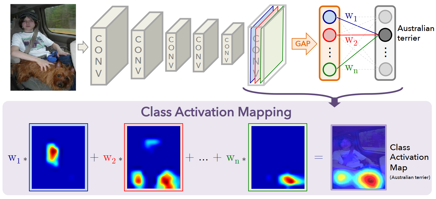
Class Activation Mapping, or CAM for short, is a special technique used in computer vision and machine learning. It helps us understand how a Convolutional Neural Network (CNN) makes decisions when classifying images. Basically, CAM lets us visualize which parts of an image are most important for the network’s prediction.

How does CAM work? #

Modify the CNN: We take a trained CNN and remove the fully connected layers at the end. Instead, we add a Global Average Pooling (GAP) layer after the last convolutional layer.
Global Average Pooling: GAP takes each feature map from the last convolutional layer and calculates the average of all values within that map. This results in a single representative value for each feature map.
Prediction with a single layer: These averaged values are then fed into a single fully connected layer with as many outputs as there are classes in our problem. This layer learns to predict the image class based on the feature map averages.
Weights and Importance: The weights in this final layer tell us how important each feature map is for each class.
Creating the heatmap: We multiply these weights with the corresponding feature maps from the last convolutional layer. This creates a weighted sum for each class, highlighting the regions in the feature maps that were most influential for that class.
Visualization: These weighted sums are then visualized as heatmaps, showing which parts of the image contributed most to the predicted class. This heatmap provides a visual explanation of the CNN’s decision-making process.

Grad-CAM #

Grad-CAM

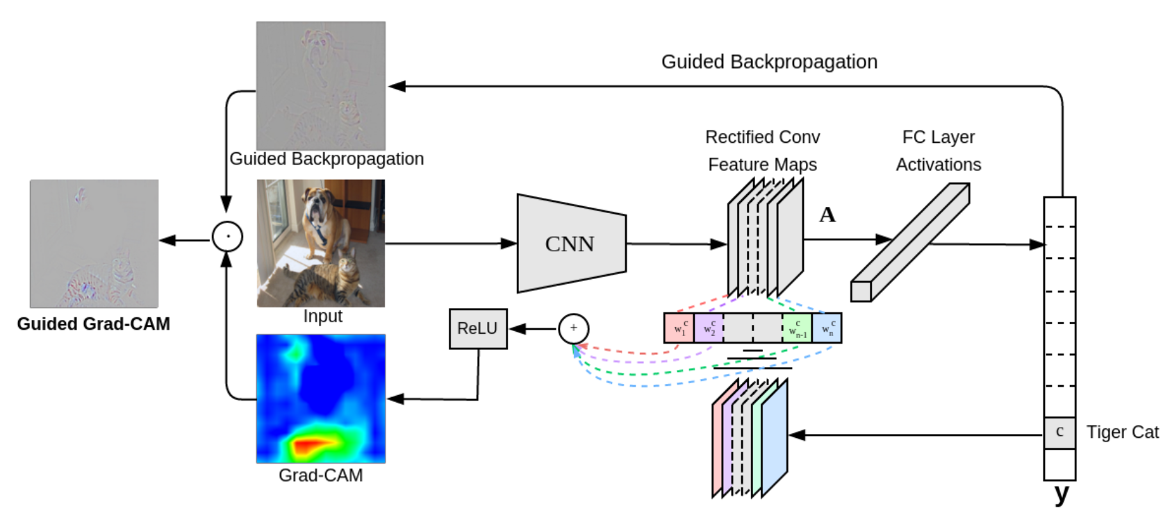
Grad-CAM, which stands for Gradient-weighted Class Activation Mapping, is another technique similar to CAM that helps us visualize what a CNN is “looking at” when making a prediction.

One key advantage of Grad-CAM is that it doesn’t require modifying the original CNN architecture, unlike CAM which needs the Global Average Pooling layer. This makes Grad-CAM applicable to a wider range of CNN models.

How does Grad-CAM work? #

Forward Pass and Prediction: We start by feeding an image into the CNN and obtaining the class prediction.
Gradient Calculation: We then calculate the gradient of the score for the predicted class with respect to the feature maps of the last convolutional layer. This tells us how much each feature map activation influences the final prediction score.
ReLU and Global Average Pooling: We apply a ReLU function to the gradients to focus on the features that have a positive influence on the class score. Then, for each feature map, we take the average of these positive gradients across all the spatial locations in that map. This gives us a single value representing the importance of each feature map for the predicted class.
Weighted Combination: We then use these averaged gradients as weights and combine them with the corresponding feature maps from the last convolutional layer. This creates a weighted sum that highlights the important regions in the feature maps for the predicted class.
Visualization as Heatmap: Finally, we visualize this weighted sum as a heatmap, superimposed on the original image. This heatmap shows which parts of the image were most influential in the CNN’s decision-making process.

Contrastive Grad-CAM Consistency Loss #

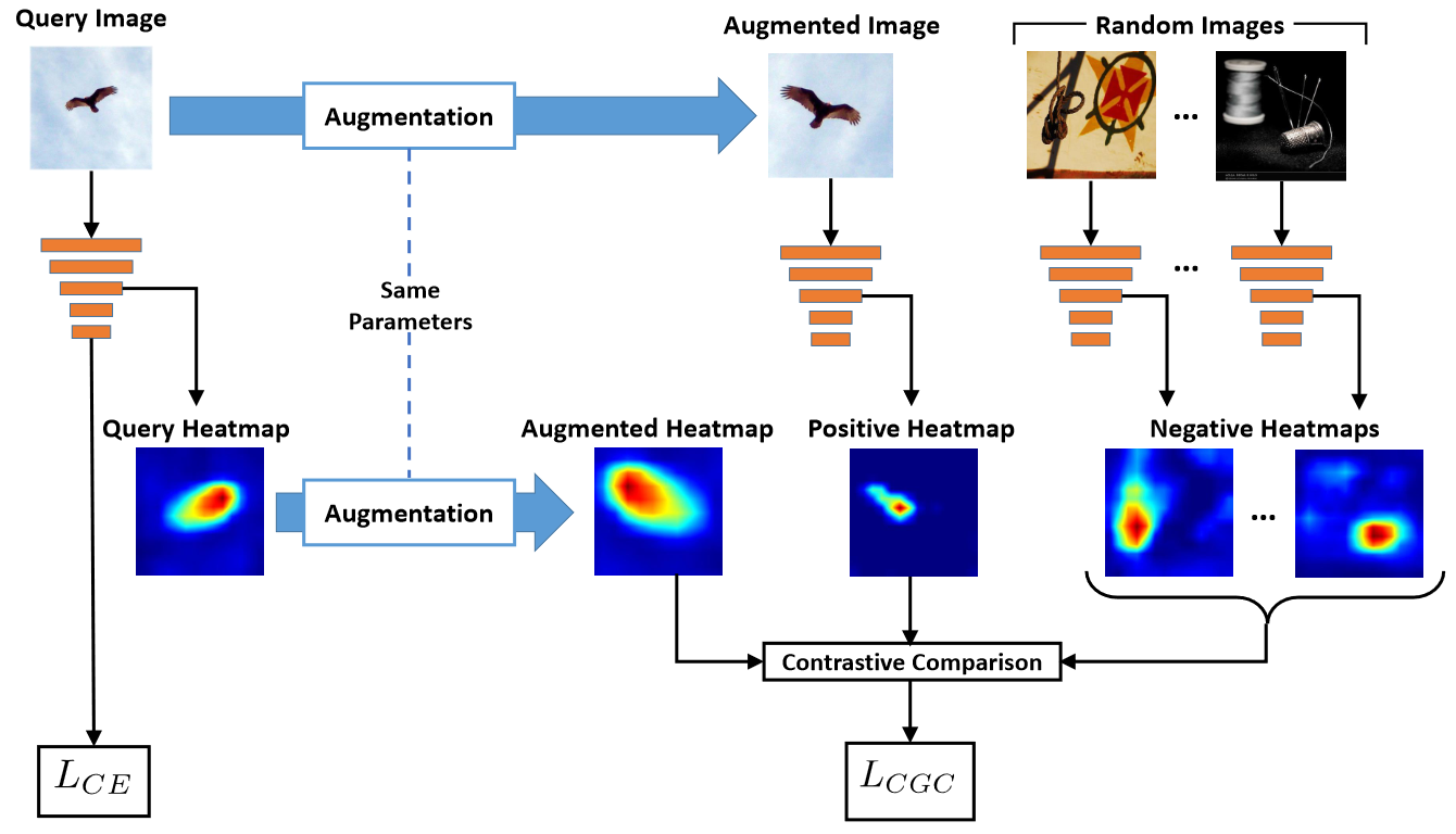
We want the transformed interpretation of a query image to be close to the interpretation of the transformed query while being far from interpretations of other random images

To understand the main formula, let’s first define the key elements involved:

\(g(\cdot)\) : Grad-CAM operator that produces interpretation heatmap
\(\{X_j\}^n_{j=1}\) : Set of \(n\) random images
\(\Tau_j(\cdot)\) : Independent random spacial transformation. This transformation could involve scaling, cropping, and/or flipping the image.
\(\{g_j(T_j(j_j))\}^n_{j=1}\) : Grad-CAM heatmaps of the augmented images
\(x_i\ where\ i\in 1..n\) : Query image
\(\Tau_i(g_i(x_i))\) : We apply the same transformation we had applied to \(x_i\) to the Grad-CAM heatmap instead of the image

We want \(\Tau_i(g_i(x_i))\) to be close to \(g_i(\Tau_i(x_i))\) and far from \(\{g_j(\Tau_j(x_j))\}_{j\neq i}\) Hence, we define the following loss function:

\[L_i = -\log{\frac{\exp(\text{sim}(\Tau_i(g_i(x_i))), g_i(\Tau_i(x_i))/\tau)}{\sum^n_{j=1}\exp(\text{sim}(\Tau_i(g_i(x_i))), g_j(\Tau_j(x_j)))}}\] where \(\tau\) is the temperature hyperparameter and \(\text{sim}(a, b)\) is a similarity function. In the experiments cosine similarity was used.

Since we want to optimize training we will assume that each image is the query once in one mini-batch. Thus we define our contrastive Grad-CAM consistency loss as: \[L_{CGC} = \sum_i{L_i}\]

Our final loss will be a combination of the cross entropy loss with defined consistency loss: \[L = L_{CE} + \lambda L_{CGC}\] where \(\lambda\) is a hyperparameter that controls trade-off between usual supervised way of training and self-supervised method that allows to train our model on unlabeled data using pseudo labels (image labels).

Here you can see visual description of the approach described above: CGC

Our Implementation #

Google Colab Notebook #

This section describes our implementation of the CGC method using PyTorch. Here’s a concise overview:

Data Loading and Transformation:
- We use the Imagenette dataset for demonstration purposes (CUB dataset is also available in the code).
- A custom ContrastiveTransforms class handles data augmentation, including random resized cropping and horizontal flips.
- Data loaders are set up for both labeled and unlabeled data.
Model Definition:
- The CGC_Model class utilizes a ResNet-18 backbone.
- A forward hook is applied to the last convolutional layer (layer4) to extract feature maps for Grad-CAM computation.
- The forward pass implements the CGC logic, including Grad-CAM calculation and augmentation.
Loss Functions and Optimization:
- We employ cross-entropy loss for supervised learning.
- The NCESoftmaxLoss (info-NCE) encourages consistency and distinctiveness in Grad-CAM heatmaps.
- SGD optimizer with momentum and weight decay is used.
Training Loop:
- The train function iterates through epochs and mini-batches, performing both supervised and contrastive learning.
- It tracks cross-entropy loss, contrastive loss, and top-1/top-5 accuracies.
Grad-CAM Visualization:
- After training, the model is loaded and used to generate Grad-CAM heatmaps for sample images.
- A display_gradcam function visualizes the original images, Grad-CAM masks, and the superimposed results.
Model Saving:
- The trained model’s state is saved for future use.