“Contrastive Explanations and Fairness in Credit Risk Predictions” #

authors:

• Aleksandra Kuzmich

Introduction #

In recent years, machine learning has become a part of decision-making pipelines in finance and banking. Models are used for a wide range of tasks, from loan approvals to credit scoring. But as these models grow in complexity, they become harder to understand. For financial institutions, relying blindly on model predictions is not acceptable. Understanding why a particular decision was made — and which features influenced is crucial.

In this tutorial, we explore how contrastive explanations and counterfactual reasoning can help uncover the decision-making process behind a credit risk prediction model.

The model we use is TabNet, introduced in 2020 in the paper TabNet: Attentive Interpretable Tabular Learning by Arik and Pfister. As of today, TabNet is no longer considered state-of-the-art in terms of raw predictive performance, but it remains a popular and practical choice, especially for interpretable deep learning on tabular data.

One of TabNet’s key features is its built-in interpretability. It uses attention-based feature masks that reveal which features were used at each decision step. This provides a baseline level of transparency, but it doesn’t answer deeper questions like:

• Why did the model make this decision instead of the other one?
• What features would need to change to get a different result?
• Is the model treating similar applicants consistently across subgroups?

Our goal is to go beyond TabNet’s built-in explanations. We’ll use contrastive logic, greedy counterfactual search, and subgroup analysis to explore not just how the model works, but whether it works fairly and sensibly.

What Are Contrastive Explanations? #

Most explainability methods try to answer: “Why did the model predict this outcome?”

Contrastive explanations flip the question:

“Why this outcome, instead of some other one?”

This small shift makes a big difference. Humans often think in contrastive terms. Like, really, we don’t usually ask why something happened in isolation. Instead, we want to know why it happened instead of what we expected.

For example: Why was this loan rejected instead of approved?

Contrastive explanations are useful because they focus only on what matters for a specific decision, ignoring everything that’s irrelevant. That makes the reasoning both more compact and more actionable.

Here we also consider identifying the minimal set of features that need to change to flip the model’s decision.

For example: If the applicant had a verified income and a slightly lower loan amount, the loan would have been approved.

This approach helps bridge the gap between black-box predictions and real-world reasoning.

Dataset #

We use real-world credit application data from the Lending Club Loan Data dataset on Kaggle. This dataset contains accepted loan applications submitted between 2007 and 2018Q4 and includes both financial and demographic attributes of borrowers.

File used: accepted_2007_to_2018Q4.csv.gz

According to the web, dataset is widely used in both academic and applied research related to:

• Credit scoring and risk modeling
• Fair lending analysis
• Automated underwriting systems
• Explainability and fairness audits in finance

It includes features such as: Annual income, Loan amount, Debt-to-income (DTI) ratio, Employment length, and more. Where by more I mean 151 column.

The target variable for our task is whether the loan was fully paid or charged off, which is viewed as “approved” or “rejected”.

Preprocessing #

For the preprocessing we:

1. Filtered relevant loan statuses to create a binary classification task
2. Handled missing values
3. Encoded categorical variables
4. Standardized numerical columns
5. Sampled 20k and split the data into 80% training and 20% testing

Model: TabNet #

To model credit risk, we use TabNet, a deep learning architecture designed specifically for tabular data. TabNet replaces traditional fully-connected layers with sequential attention-based feature selection, allowing the model to focus on different subsets of features at each decision step.

We trained the model using the pytorch-tabnet library with the following setup:

• Optimizer: Adam with a moderately aggressive learning rate
• Training duration: Up to 50 epochs with early stopping based on validation accuracy
• Batching: Large batch size with smaller virtual batches to regularize learning

The model was trained on a binary classification task: predicting whether a loan would be fully paid or charged off. After training, it achieved good performance on the test set, with precision and recall above baseline levels for both classes (above 95%).

Start of XAI analysis #

Feature Dictionary #

• total_rec_prncp: Total loan principal repaid
• last_pymnt_amnt: Amount of the most recent payment
• last_fico_range_low: Lower bound of the latest FICO score range
• last_pymnt_d: Date of the last payment
• last_credit_pull_d: Date of last credit check
• issue_d: When the loan was issued
• earliest_cr_line: Date of the borrower’s first credit line
• addr_state: State of residence
• emp_length: Length of employment
• last_fico_range_high: Upper bound of latest FICO range
• percent_bc_gt_75: % of credit cards with high balances
• revol_util: % of revolving credit used
• mths_since_recent_inq: Months since last credit inquiry
• total_bc_limit: Total credit limit across all bankcard accounts
• bc_open_to_buy: Remaining credit on open bankcard accounts
• application_type: Indicates if the application is individual or joint
• debt_settlement_flag: Whether the borrower has settled debt for less than owed
• num_tl_90g_dpd_24m: Number of tradelines (loans/credit lines) with 90+ days past due in the past 24 months

Visualizing Contrastive Features #

After generating contrastive explanations, we aggregate the results to identify which features most often contributed to flipping a decision. This provides insight into the most influential features for each class.

Below are two horizontal bar plots showing the top contrastive features for:

• Charged-Off loans (predicted defaults)
• Fully Paid loans (successful repayments)

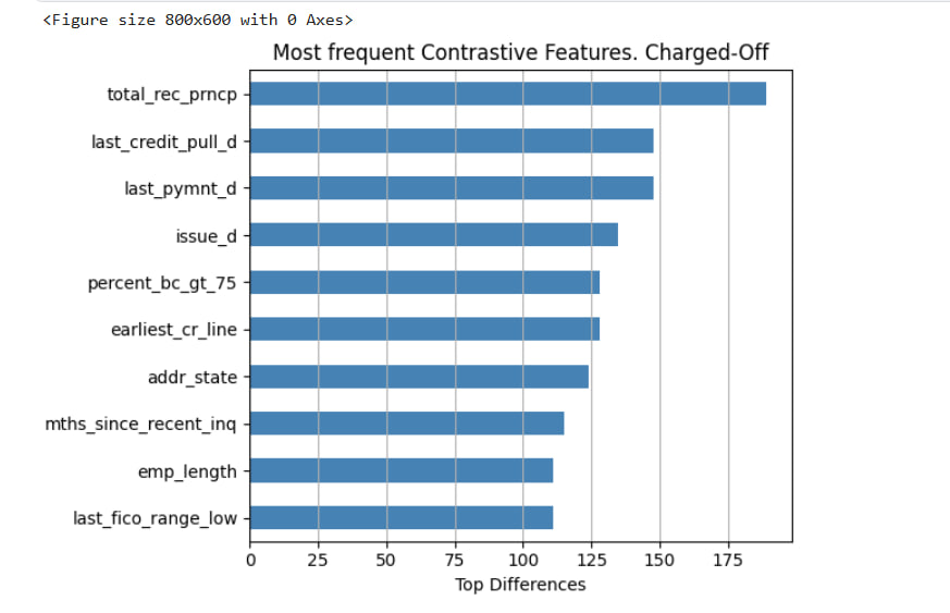
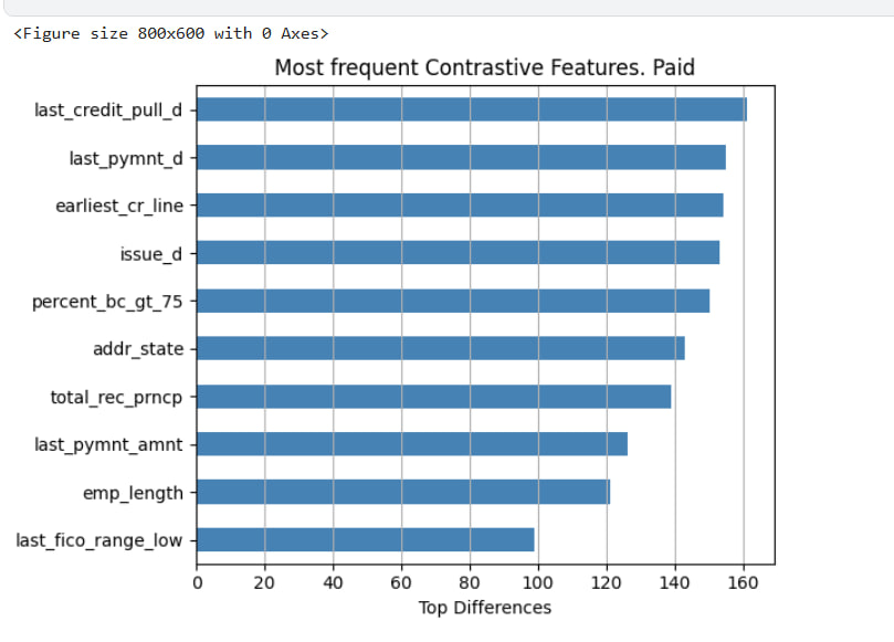
These plots reflect which features most frequently differed between a sample.

Key Observations #

• Features related to payment timing (e.g., last_pymnt_d, last_credit_pull_d) and credit history (e.g., earliest_cr_line, issue_d) show up in both classes.
• total_rec_prncp (total principal received) is highly contrastive in Charged-Off cases, suggesting the model often associates low repayment with risk.
• last_pymnt_amnt and total_bc_limit appear only for Fully Paid cases, possibly indicating that the model pays more attention to available revolving credit when assessing lower-risk applicants.

Comparing Contrastive Sets #

To better understand how the model treats different classes, we built a table comparing the features that appear exclusively in one class, shared between both, or are unique to the other.

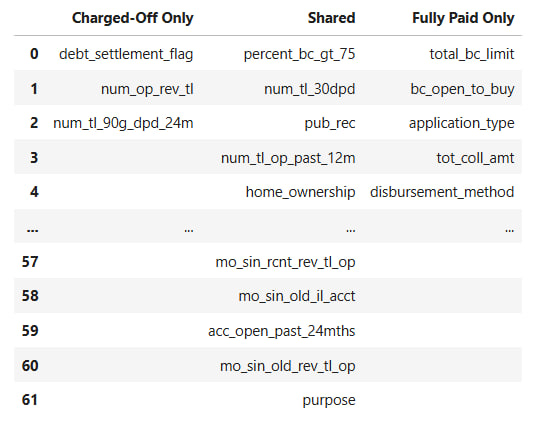
Features debt_settlement_flag or num_tl_90g_dpd_24m are only contrastive for Charged-Off loans, aligning with higher-risk borrower profiles. Conversely, application_type, bc_open_to_buy, and total_bc_limit are unique to Fully Paid cases, potentially reflecting stronger financial standing.

Fairness Through Contrastive Explanations #

One of the strengths of contrastive explanations is that they can reveal how a model reasons about different subgroups. In this section, we investigate whether TabNet’s predictions of loan default “Charged-Off” depend on different features for different types of applicants.

We break applicants down into two dimensions:

• Income group: High vs. Low, based on median annual income.
• Verification status: Whether the applicant’s income was Verified, Partially Verified, or Not Verified.

By Income Group #

We generated contrastive explanations for Charged-Off predictions from both High Income and Low Income groups. The tables below show which features most frequently contributed to flipping a prediction — in other words, which features differentiated Charged-Off applicants from otherwise similar Fully Paid applicants.

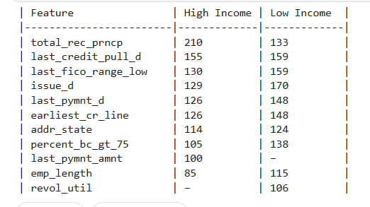
We observe some notable differences:

• Features like total_rec_prncp, last_pymnt_amnt, and last_fico_range_low appear more frequently in High Income explanations.
• Meanwhile, revol_util and percent_bc_gt_75 were more common contrastive factors among Low Income applicants.

These patterns suggest that the model uses different signals to justify risk across income levels even when predicting the same outcome.

By Verification Status #

We repeated this analysis for income verification status. Again, we sampled predictions from each group: Verified, Partially Verified, and Not Verified.

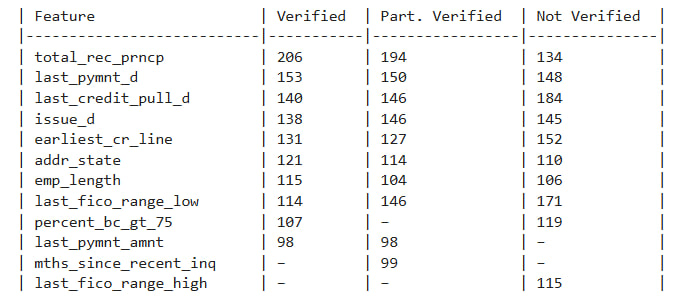
The differences here are even more striking:

• For Verified applicants, contrastive features leaned heavily on repayment history (total_rec_prncp, last_pymnt_d, etc.).
• For Not Verified applicants, features like last_fico_range_high and percent_bc_gt_75 were more influential, suggesting the model may be more cautious in the absence of income documentation.

These findings don’t imply discrimination but they do reveal asymmetries in how the model makes decisions for different groups.

Counterfactual Explanations #

To understand how sensitive the model is to individual features, we implemented a greedy counterfactual search. The goal is to answer the question:

What’s the smallest set of changes we can make to flip the model’s prediction?

We focused on samples predicted as Fully Paid (Class 0), and tried to change them into Charged-Off (Class 1) by incrementally tweaking one feature at a time. The search stops once the prediction flips or no combination works.

Most Frequently Changed Features #

The bar chart below shows which features were most often changed across samples:

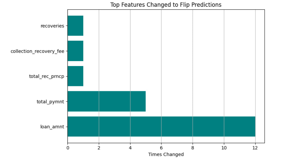
Samples requiring more changes are likely closer to the model’s decision boundary. Unflippable cases suggest high model confidence in the original prediction.

These are the features the model relies on most when reconsidering its decision. loan_amnt, in particular, appears highly influential in flipping predictions from low to high risk.

This kind of analysis is useful when considering actionability, it tells not just what features mattered, but which changes would actually make a difference.

Extra! SHAP jumpscare #

While contrastive explanations tell us what sets examples apart, SHAP shows which features actually pushed the decision one way or the other.

We implemented a simplified version of SHAP from scratch. For each feature, we compute the model’s output with and without that feature (using a baseline value in its place), then average the marginal contribution across random subsets.

Single Prediction #

Since the whole ivestigation is time expensive, we applied this method to one sample predicted as Fully Paid. Features with negative SHAP values reduced the predicted risk (pushed toward approval), while positive values pushed the prediction toward Charged-Off.

Fairness Audit #

To investigate fairness, we extended the SHAP approach to compare average feature attributions across demographic subgroups. Income and verification, as in previous example. For each group, we sampled examples, computed SHAP values, and averaged them to reveal the top influencing features.

What obtained? #

Since the SHAP part was a bit of an afterthought (and the implementation isn’t optimized), we didn’t run a full-blown analysis on the entire dataset. Still, a few sample explanations were enough to show that the model uses different signals depending on income and verification status, which already tells us something interesting.

Results and future Work #

Contrastive explanations helped pinpoint which features separate approved from rejected applicants. Using feature frequency across contrastive matches, we saw clear patterns: the model uses different signals for different classes and subgroups. Fairness analysis revealed that even when predicting the same outcome, the model looks at different features for high- vs. low-income users or verified vs. unverified ones.

Next #

• Improve the efficiency of SHAP
• Add more counterfactual metrics, like distance or plausibility scoring, to go beyond basic flips.
• Try other fairness criteria.
• Most of the explanations were done for just one class (Charged-Off). That was mainly for time and clarity. But in a full study, we’d absolutely want to repeat everything for the opposite class too to make sure the model isn’t only explainable or fair in one direction.

GitHub Link #

Check notebook