Counterfactual Explanations for Credit Risk Models: A Case Study #
TL;DR #
In this case study, we implement and incrementally refine a gradient-based approach for generating counterfactual explanations in credit risk modeling. Beginning with a basic optimization procedure, we identify and resolve multiple real-world issues:
- Immutable and semantically constrained features
- Inter-feature dependencies (e.g., derived ratios)
- Ordinal variables that require discrete treatment
- One-hot encoded categorical features that demand joint behavior
We develop solutions involving gradient masking, differentiable approximations, manual feature injection, and the Gumbel-Softmax trick to ensure our counterfactuals are not only effective, but valid, interpretable, and realistic.
1. Introduction: What Are Counterfactual Explanations? #
Given a binary classifier \( f(\mathbf{x}) \) trained to predict whether a loan applicant will default, counterfactual explanations aim to answer:
“What minimal changes to the applicant’s features would have changed the model’s decision?”
This is framed as an optimization:
\[\min_{\mathbf{x}'} \; d(\mathbf{x}, \mathbf{x}') + \lambda \,\mathcal{L}(f(\mathbf{x}'), c)\]Where:
- \( \mathbf{x} \) : original input (e.g., borrower profile)
- \( \mathbf{x}' \) : counterfactual
- \( d(\cdot) \) : distance measure (e.g., \( L_2 \) )
- \( \mathcal{L} \) : classification loss (e.g., binary cross-entropy)
- \( c \) : desired target label (e.g., “non-default”)
- \( \lambda \) : hyperparameter for trade-off
This setup seeks small yet decisive modifications leading to a different prediction.
2. Feature Overview and Data Constraints #
Below is a portion of the feature table, which highlights which attributes are editable and which must be constrained:
| Feature | Type | Editable? | Notes |
|---|---|---|---|
person_age | Numerical | No | Immutable personal attribute |
person_income | Numerical | Yes | Editable under assumptions like increased reported income |
loan_amnt | Numerical | Yes | Can be adjusted in application |
loan_percent_income | Derived | No (recalculated) | Must reflect ratio \( \frac{\text{loan}}{\text{income}} \) |
person_home_ownership | Ordinal | Yes | Must remain integer in range \([0,3]\) |
loan_intent_* | One-hot | No | User-declared purpose; not editable |
loan_grade_* | One-hot | No | Lender-assigned; immutable |
cb_person_default_on_file_* | One-hot | No | Historical; immutable |
3. Baseline Counterfactual Optimization #
Our initial approach used unconstrained gradient descent to find \( \mathbf{x}' \) :
x_cf = x_original.clone().requires_grad_(True)
optimizer = torch.optim.Adam([x_cf])
The loss combined:
- Distance: \( \| \mathbf{x}' - \mathbf{x} \|_2 \)
- Prediction: BCE loss w.r.t. the desired label
Result Example #
For a loan applicant predicted to default, the method produced a counterfactual flipping the label to non-default by nudging:
| Feature | Original | Counterfactual | Δ |
|---|---|---|---|
person_income | 0.0147 | 0.0141 | -0.0006 |
loan_amnt | 0.0956 | 0.1076 | +0.0119 |
Conceptually effective — but many invalid changes appeared in derived, ordinal, and categorical features.
4. Maintaining Derived Feature Consistency #
Problem #
We expected:
\[\text{loan\_percent\_income} = \frac{\text{loan\_amnt}}{\text{person\_income}}\]But after checking with:
assert np.allclose(data['loan_amnt'] / data['person_income'], data['loan_percent_income'])
We received an AssertionError.
Root Cause #
The discrepancy arose from independent MinMax scaling. Since each variable was normalized individually:
\[x_{\text{scaled}} = \frac{x - x_{\min}}{x_{\max} - x_{\min}}\]the relationship:
\[\frac{\text{scaled\_loan}}{\text{scaled\_income}} \neq \text{scaled\_loan\_percent\_income}\]Solution #
To preserve consistency, we:
- Inverse-transform
loan_amntandperson_incomefrom \([0,1]\) to real domain - Recompute: \[ r = \frac{\text{loan\_amnt}}{\text{income}} \]
- Re-scale \(r\) into \([0,1]\)
- Inject this back into the
loan_percent_incomecolumn
This is done after every optimizer step. The feature remains frozen during training, but dynamically updated to reflect valid relationships.
Example #
| Feature | Original | Counterfactual | Δ |
|---|---|---|---|
loan_percent_income | 0.1424 | 0.1635 | +0.0211 |
Shows a recalculated, updated value consistent with other features.
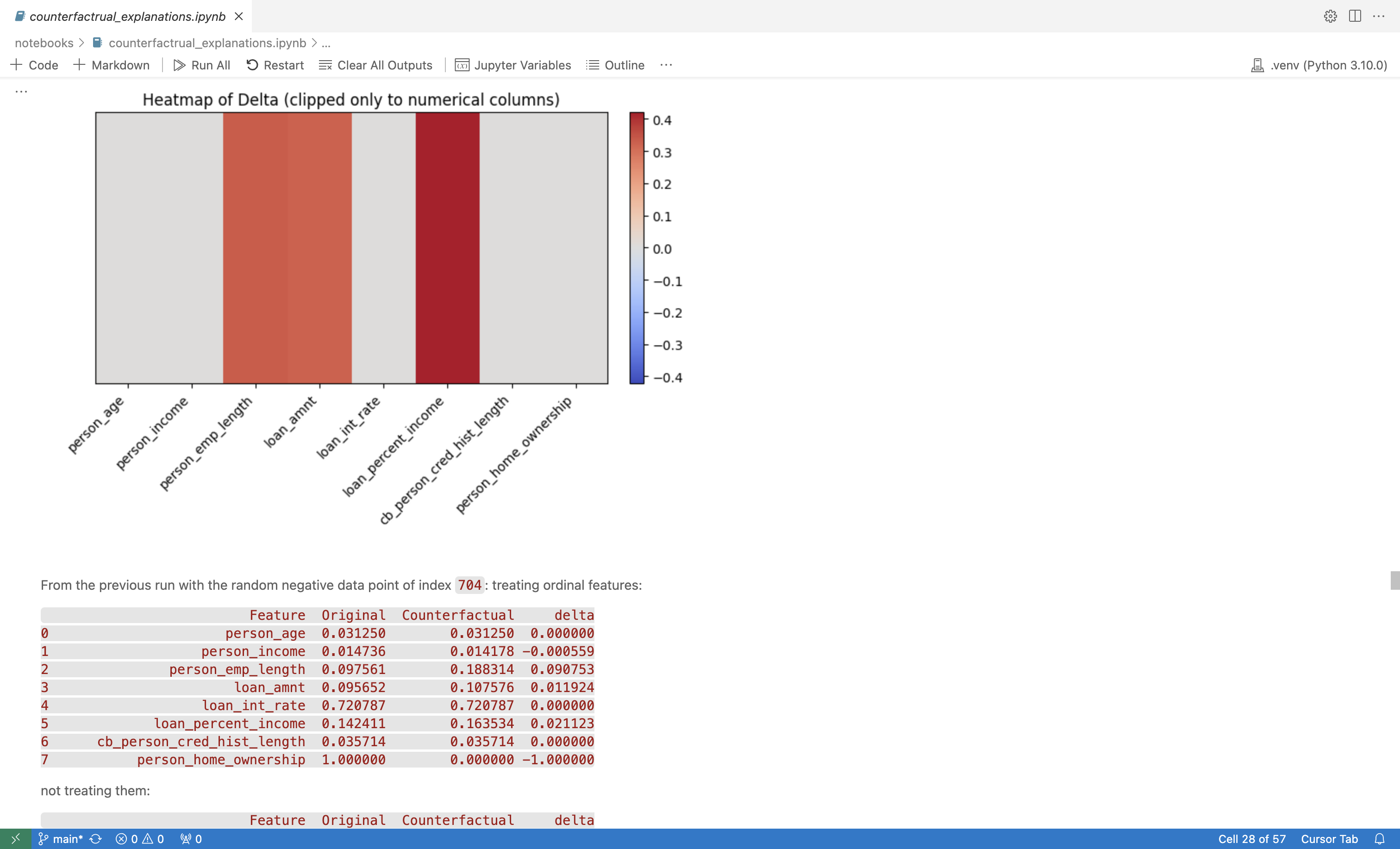
5. Treating Ordinal Features Correctly #
Problem #
Features like person_home_ownership are stored as integers (e.g., 0 = RENT, 1 = MORTGAGE). During unconstrained optimization, we observed invalid intermediate values:
| Feature | Original | Counterfactual |
|---|---|---|
person_home_ownership | 1.0000 | 0.5095 |
The model was never trained on fractional values — leading to unpredictable behavior.
Solutions #
A. Snapping #
After each step:
\(x_{\text{ordinal}} = \text{round}(x_{\text{ordinal}})\)Ensures the feature stays valid, but introduces discontinuities in gradients.
B. Soft-Round Penalty #
We added a soft penalty to the loss:
\(\alpha \sum_{i \in \text{ordinals}} \left| x_i - \text{soft\_round}(x_i) \right|\)Where:
\(\text{soft\_round}(x) = \lfloor x \rfloor + \sigma\left( \beta(x - \lfloor x \rfloor - 0.5) \right)\)- Smooth approximation to rounding
- Allows gradient descent to work effectively
Final Output #
After optimization, we snap to the nearest integer to guarantee validity.
Example #
| Feature | Original | Counterfactual | Treated | Untreated |
|---|---|---|---|---|
person_home_ownership | 1.0000 | 0.0000 | ✅ Yes | 0.5095 |
6. Ensuring Valid One-Hot Encoded Categorical Features #
Initial Misstep #
Initially, we treated each one-hot column independently — for instance:
loan_intent_EDUCATION,loan_intent_MEDICAL, etc., were optimized separately.
This created invalid one-hot groups like:
EDUCATION: 0.22
PERSONAL:  0.39
MEDICAL:   0.19
VENTURE:   0.20
This is not a valid categorical state, since:
- More than one entry ≠ 1.0
- Their sum ≠ 1.0
- The model was never trained on such combinations
Desired Behavior #
If one value in a one-hot group is increased (e.g., MEDICAL from 0 → 1), all others should go to 0. In other words:
\(\sum_{j=1}^K x_j = 1, \quad x_j \in \{0, 1\}\)Solution: Gumbel-Softmax Trick #
We reformulate the optimization problem using logits \( \boldsymbol{\pi} \) instead of directly optimizing one-hot vectors.
Each one-hot group is represented as:
\(\mathbf{y} = \text{softmax}\left( \frac{\log \boldsymbol{\pi} + \mathbf{g}}{\tau} \right)\)Where:
- \( \mathbf{g} \sim \text{Gumbel}(0, 1) \) : random noise
- \( \tau \) : temperature parameter
During training:
- \( \mathbf{y} \in [0,1]^K \)
- \( \sum y_i = 1 \)
- Behaves like a softened categorical distribution
At Inference #
After optimization:
\(\mathbf{y}_{\text{final}} = \text{one\_hot}(\arg\max_i \pi_i)\)We recover a valid one-hot vector for model input and interpretation.
Example #
# Before optimization
[1, 0, 0, 0, 0, 0]  # PERSONAL

# After optimization (logits + Gumbel)
[0.25, 0.25, 0.05, 0.40, 0.05, 0.00]  # Soft

# Final snapped output
[0, 0, 0, 1, 0, 0]  # MEDICAL
The result is a valid category shift, suitable for generating counterfactuals in exploratory settings.
7. Full Optimization Pipeline #
At each iteration: #
Forward pass:
- Compute model prediction
- Compute distance loss
- Add penalties (e.g., soft-round)
Backward pass:
- Apply gradient mask to immutable features
Step:
- Perform
optimizer.step()
- Perform
Post-processing:
- Recompute derived features (e.g., ratios)
- Inject into
x_cf - Apply soft-round or snapping to ordinal features
- Apply Gumbel-softmax projection to categorical groups
8. Summary of Techniques #
| Feature Type | Issue | Solution |
|---|---|---|
| Derived ratio | Invalid dependency | Manual recomputation + injection |
| Ordinal (int, 0–3) | Fractional output | Soft-round penalty + final rounding |
| One-hot categorical | Soft invalid combinations | Gumbel-softmax + snapping |
| Frozen features | Should not change | Gradient masking |
9. Technical Implementation #
The practical implementation of the concepts discussed in this report can be explored through our open-source repository. The repository contains all the necessary code, configurations, datasets, and interactive notebooks required for replicating our results.
GitHub Repository:
🐈⬛ Link
Repository Structure #
The repository is structured clearly to facilitate easy navigation and reproducibility of the results:

Notebooks #
The notebook counterfactual_explanations.ipynb provides an interactive and detailed step-by-step walkthrough of the counterfactual generation process, illustrating clearly how each technique from gradient masking to Gumbel-softmax is applied.

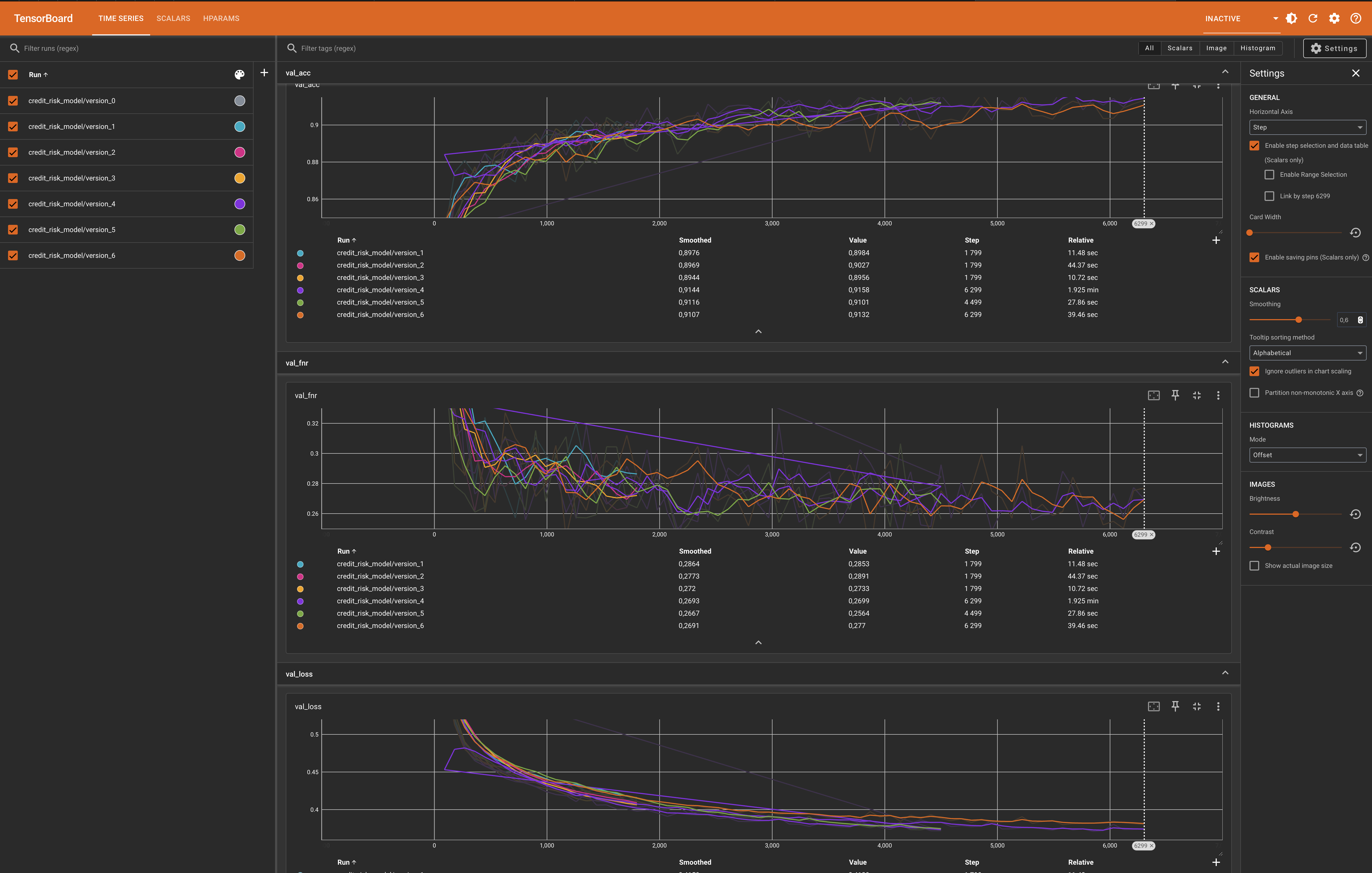
Model Training Visualization #
During the training phase, we monitored the model’s performance metrics using TensorBoard, enabling us to fine-tune the hyperparameters and verify convergence effectively.
Deployment #
To make our approach interactive and accessible, we have implemented a deployment pipeline using Streamlit. After obtaining the trained model weights and updating configuration files, users can deploy the application locally by running:
bash deploy.sh
This will launch a Streamlit app that enables interactive exploration of counterfactual explanations.


The interactive deployment provides users with an intuitive interface to explore how changes in feature values affect predictions, thus demonstrating the practical applicability and interpretability of our method.
10. Conclusion #
This case study demonstrates how to go from a naive counterfactual optimizer to a realistic, interpretable system that respects domain logic and data semantics.
By:
- Freezing immutable features
- Respecting feature relationships
- Maintaining categorical validity
- Applying differentiable approximations
we move toward counterfactuals that are both accurate and meaningful — critical for high-stakes domains like finance and credit.
References #
Counterfactual Explanations:
Wachter, S., Mittelstadt, B., & Russell, C. (2018).
Counterfactual explanations without opening the black box: Automated decisions and the GDPR.
Harvard Journal of Law & Technology, 31(2), 841–887.
https://arxiv.org/abs/1711.00399Gumbel-Softmax Trick for Differentiable Sampling:
Jang, E., Gu, S., & Poole, B. (2017).
Categorical reparameterization with Gumbel-Softmax.
International Conference on Learning Representations (ICLR).
https://arxiv.org/abs/1611.01144Soft-Rounding (Differentiable Approximation):
Agustsson, E., & Theis, L. (2020).
Universally Quantized Neural Compression.
Advances in Neural Information Processing Systems (NeurIPS), 33, 12367–12376.
https://arxiv.org/abs/2006.09952