Diffusion Lens: Interpreting Text Encoders in Text-to-Image pipelines #
Authors: Ivan Golov, Roman Makeev
To see the implementation, visit our github project.
Introduction #
In this work, we introduce an interpretable, end-to-end framework that enhances Stable Diffusion v1.5 model fine‑tuned via the DreamBooth method [1] to generate high‑fidelity, subject‑driven images from as few reference examples.
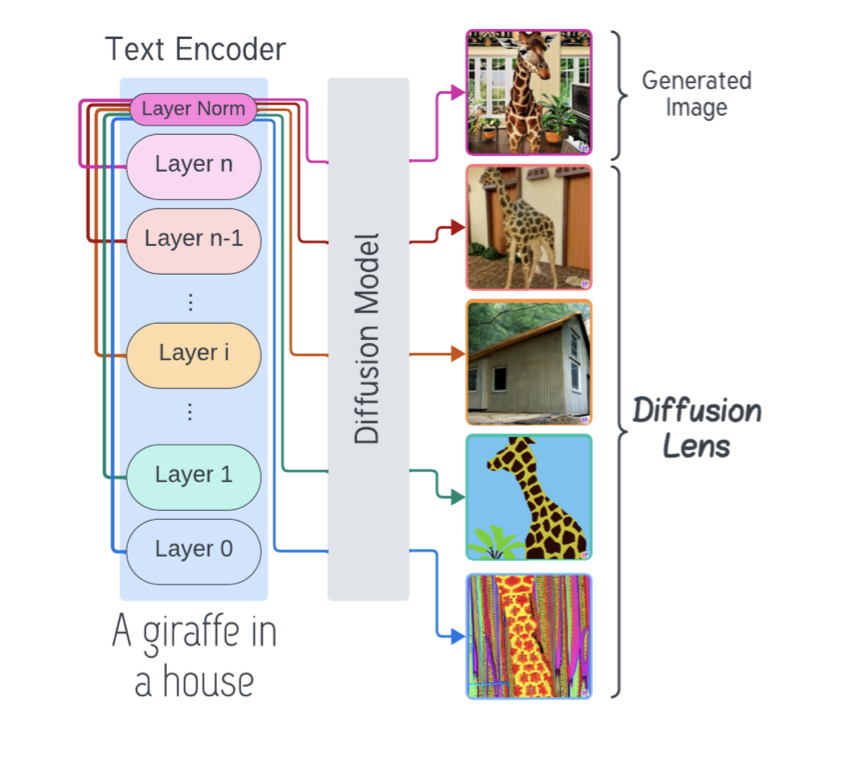
While DreamBooth effectively personalizes generation by associating a unique rare token with the target concept, the internal process through which textual prompts are transformed into visual representations remains opaque. To bridge this gap, we integrate Diffusion Lens [2], a visualization technique that decodes the text encoder’s intermediate hidden states into images, producing a layer‑by‑layer sequence that illuminates how semantic concepts emerge and refine over the course of encoding.
Background #
Section 1: DreamBooth Fine-Tuning #
DreamBooth [1] fine-tunes a pre-trained diffusion model with a small set (3–5) of images of a subject by binding a unique, rare-token identifier to the subject. The rare token, chosen from the text encoder’s vocabulary, acts as a minimal prior and is used to encode target image features and styles. The main training objective is given by:
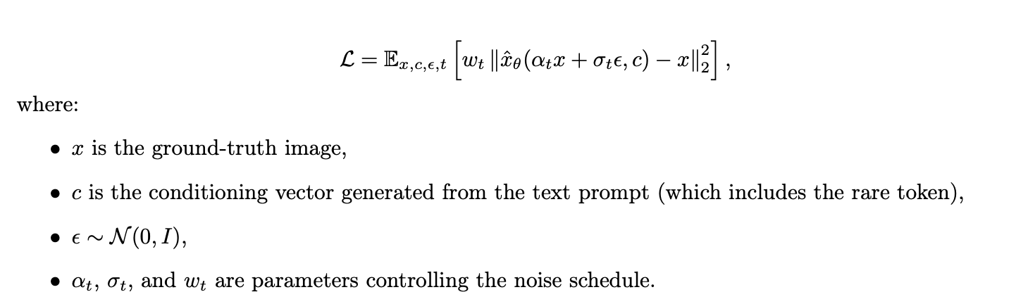
An additional prior preservation loss ensures that the model retains its generalization over the subject’s class even after fine-tuning.
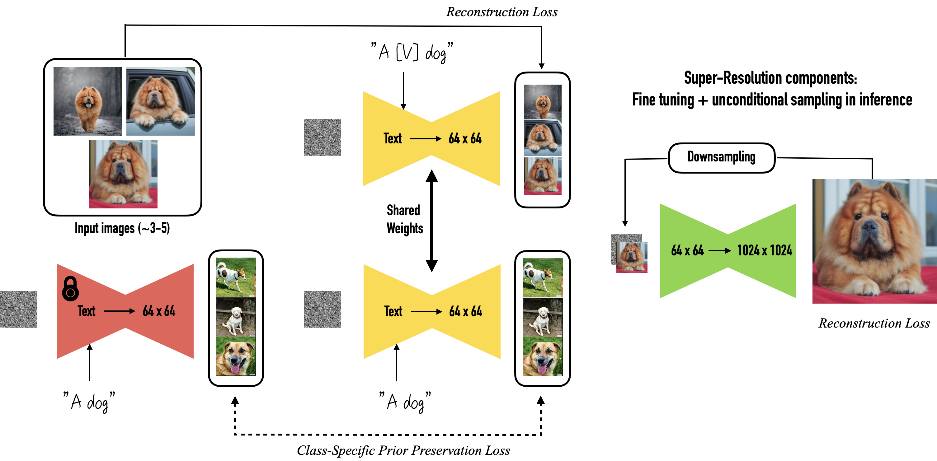
Figure 1: Illustration of the DreamBooth approach: Fine-tuning the diffusion model using rare tokens to encode target subject details and style
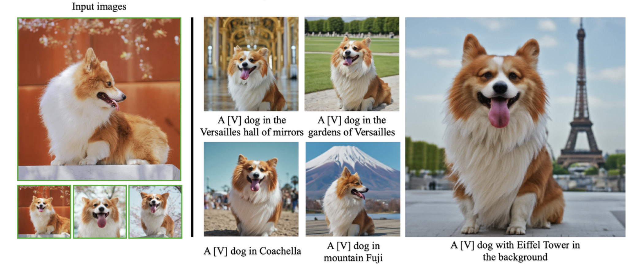
Figure 2: Expected output from DreamBooth fine-tuning: Images generated that exhibit the target subject details and stylistic features as encoded by the rare tokens.
Section 2: Diffusion Lens Interpretability #
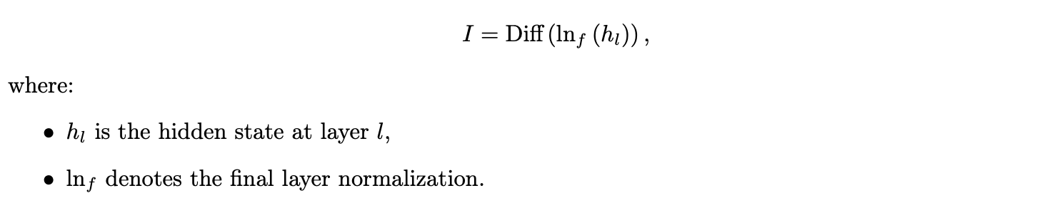
Diffusion Lens [2] is employed to analyze the internal representations of the text encoder after the fine-tuning process. Rather than solely relying on the final output, we generate images from intermediate hidden states. For a given layer l (with l < L for a total of L layers), the generated image is:
This method provides:
- Layer-by-Layer Understanding: Early layers capture basic, unstructured representations (a “bag of concepts”), while later layers progressively refine and organize these ideas.
- Complexity Analysis: Simple prompts (e.g., “a cat”) yield clear representations in early layers, whereas complex prompts (e.g., “a red car next to a blue bike”) require deeper layers to form accurate relational structures.
- Concept Frequency Insights: Common concepts appear early, uncommon or detailed concepts emerge only in higher layers.
- No Extra Training Required: The analysis leverages the pre-trained model without modifying its architecture
Methodology #
3.1 Codebase Organization #
Our project is structured to separate main modules and scripts:
GAI_course_project/
├── configs/                 # YAML/JSON configs for training and inference
├── data/                    # Raw and preprocessed datasets
├── DiffusionLens/           # Core implementation of Diffusion Lens pipeline
├── inference_outputs/       # Generated images and logs from inference runs
├── lens_output/             # Intermediate visualizations produced by Diffusion Lens
├── LICENSE
├── notebooks/               # Experiment notebooks
│   ├── Diffusion_Lens_framework.ipynb
│   ├── Experiment№1_token_understanding.ipynb
│   ├── Experiment№2_latent_representations.ipynb
│   ├── Text_Encoder_Architecture_exploration.ipynb
│   └── README.md
├── outputs/                 # Final sample images and metrics
├── papers/                  # PDF versions of referenced papers
├── poetry.lock              # Dependency lockfile
├── pyproject.toml           # Package definition
├── README.md
├── requirements.txt         # pip dependencies
├── scripts/                 # Utility scripts (data download, env setup ... )
├── src/                     # Main training and evaluation code
└── static/                  # Fixed assets (figures, math images)
3.2 Text Encoder Architecture #
We use the Hugging Face CLIPTextModel from sd-legacy/stable-diffusion-v1-5:
CLIPTextModel(
  text_model=CLIPTextTransformer(
    embeddings=CLIPTextEmbeddings(
      token_embedding: Embedding(49408, 768)
      position_embedding: Embedding(77, 768)
    ),
    encoder=CLIPEncoder(layers=[12 × CLIPEncoderLayer]),
    final_layer_norm=LayerNorm(768)
  )
)
Each of the 12 CLIPEncoderLayercomprises:
- Multi‑head self‑attention (
q_proj,k_proj,v_proj,out_proj) - LayerNorm (pre‑ and post‑MLP)
- MLP (
fc1→ QuickGELU →fc2)
We extract the hidden state simply by advancing the input through the transformer stack and collecting the intermediate outputs.
3.3 Diffusion Lens Pipeline Setup #
The Diffusion Lens Pipeline extends Hugging Face’s StableDiffusionPipeline into StableDiffusionGlassPipeline, adding two key interpretability hooks:
- Text‑encoder split via
start_layer: index of first CLIP layer to decodeend_layer: (exclusive) index of last layer to decodestep_layer: stride between layers
- U‑Net snapshot via
callback(step, timestep, latents)callback_steps: interval of denoising steps at which to invokecallback
from DiffusionLens.pipeline import StableDiffusionGlassPipeline

# 1. Instantiate the pipeline
pipe = StableDiffusionGlassPipeline(
    vae=vae,
    text_encoder=text_encoder,
    tokenizer=tokenizer,
    unet=unet,
    scheduler=scheduler,
    safety_checker=None,
)
pipe.to(DEVICE)

# 2. Run with interpretability hooks
layer_outputs = pipe(
    prompt="A red sports car",          # or List[str]
    negative_prompt="low resolution",   # optional
    num_inference_steps=50,
    guidance_scale=7.5,
    generator=generator,                # torch.Generator for reproducibility
    num_images_per_prompt=1,
    start_layer=0,                      # decode from layer 0
    end_layer=12,                       # up to layer 11
    step_layer=2,                       # every 2 layers
    output_type="pil",                  # "pil" or "latents"
    return_dict=True,
    callback=unet_latent_hook,          # function to capture U‑Net latents
    callback_steps=10,
    cross_attention_kwargs=None,
    guidance_rescale=0.0,
    skip_layers=None,
    explain_other_model=False,
    per_token=False,
)
Available arguments (beyond the standard diffusion settings listed above):
- prompt (
strorList[str]): text to guide image synthesis - height, width (
int, optional): output resolution (defaults tounet.config.sample_size * vae_scale_factor) - negative_prompt (
strorList[str]): steer away from unwanted content - generator (
torch.Generator): for deterministic sampling - latents (
torch.FloatTensor, optional): pre‑sampled latents to reuse - prompt_embeds, negative_prompt_embeds (
torch.FloatTensor, optional): bypass tokenization - return_dict (
bool): return aStableDiffusionPipelineOutputifTrue, else a tuple - cross_attention_kwargs (
dict, optional): e.g.,{"scale": LoRA_scale} - guidance_rescale (
float): adjust classifier‑free guidance strength - skip_layers (
List[int], optional): explicitly skip certain CLIP layers - explain_other_model (
bool): enable cross‑model comparison mode - per_token (
bool): decode embeddings for each token separately
With these settings, a single call to pipe(...) will produce both:
- A sequence of images, one per text‑encoder layer;
- Optionally, U‑Net latent snapshots, captured via your
callback.
3.4 Unified Layer‑wise Decoding & Latent Snapshotting #
Below is a distilled pseudo‑code sketch of single‑pass interpretability routine:
def __call__(..., start_layer=0, end_layer=-1, step_layer=1,
             callback=None, callback_steps=1, ...):
    """
    For each selected text‑encoder layer ℓ:
      • Encode prompt up to ℓ → partial embedding.
      • Run diffusion denoising with that embedding.
      • During denoise, if (step % callback_steps == 0): callback(...)
      • Decode final latents → PIL image.
    Returns all layer‑wise images (and any latents via callback).
    """
    # 1. Input validation
    self.check_inputs(...)

    # 2. Split prompt into embeddings_per_layer
    embeddings = self._encode_prompt(
        prompt, start_layer, end_layer, step_layer, ...
    )

    images = []
    for ℓ, embed in enumerate(embeddings):
        # 3a. Initialize scheduler & latents
        self.scheduler.set_timesteps(num_inference_steps, device)
        latents = self.prepare_latents(...)

        # 3b. Denoising loop
        for step, t in enumerate(self.scheduler.timesteps):
            lat_in = (
                torch.cat([latents]*2)
                if guidance_scale>1 else latents
            )
            lat_in = self.scheduler.scale_model_input(lat_in, t)
            noise = self.unet(lat_in, t, encoder_hidden_states=embed)[0]
            if guidance_scale>1:
                uncond, text = noise.chunk(2)
                noise = uncond + guidance_scale*(text-uncond)
            latents = self.scheduler.step(noise, t, latents)[0]

            if callback and step % callback_steps == 0:
                callback(step, t, latents)

        # 3c. Decode & collect image
        img = self.vae.decode(latents / self.vae.config.scaling_factor)[0]
        images.append(self.image_processor.postprocess(img, output_type, [True]))

    # 4. Return images (plus any capture via callback)
    return images
Why this matters:
- Text‑encoder decoding reveals when concepts (objects, colors, relations) emerge.
- U‑Net snapshots show how DreamBooth’s subject details are injected over diffusion steps.
- Single invocation keeps training/inference overhead minimal and ensures full end‑to‑end traceability.
Note: For further details, please see our notebooks/Diffusion_Lens_framework.ipynb notebook and the official
Diffusion Lens GitHub repository.
Experiments and Analysis #
1. DreamBooth Explainability During Training #
Objective: #
To understand how fine-tuning with the DreamBooth approach alters the internal representations of the Stable Diffusion model during training, we use DiffusionLens to visualize the evolution of the text encoder layers over time.
Setup: #
- Model:
runwayml/stable-diffusion-v1-5 - Unique identifier:
xon - Instance prompt:
"a photo of xon dog" - Class prompt:
"a photo of a dog" - Negative prompt:
"low quality, blurry, deformed" - Visualization tool:
DiffusionLens - Visualization frequency: Every 50 epochs (from 50 to 350)
- Layers analyzed: Text encoder layers 0 to 12
Config Snapshot: #
We used the following config file: configs/train_dog_dreambooth_with_lens.yaml, with key parameters such as:
train_text_encoder: truenum_train_epochs: 350use_diffusion_lens: truediffusion_lens_epochs: 50
Procedure: #
- The model is trained using DreamBooth with a personalized prompt format.
- Every 50 epochs, DiffusionLens is used to extract and visualize activations from each layer of the text encoder.
- Layers 0 through 12 are analyzed to observe changes in learned representations.
Text Encoder Layer Evolution During DreamBooth Training #
Layer 0 Layer 1 Layer 2
Layer 3 Layer 4 Layer 5
Layer 6 Layer 7 Layer 8
Layer 9 Layer 10 Layer 11
Layer 12 (Final styled output)
Insights #
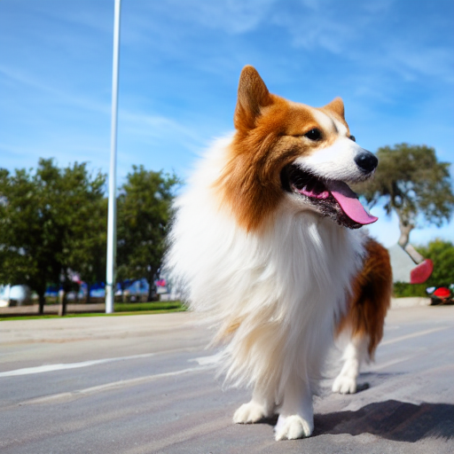
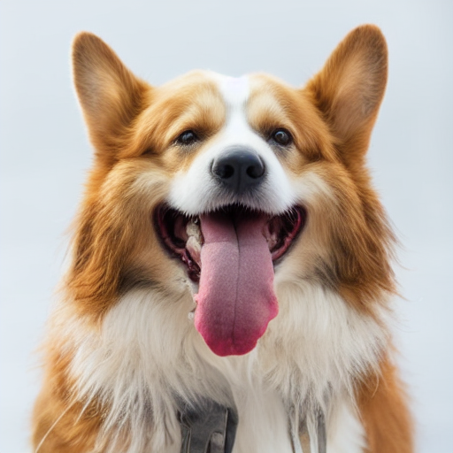
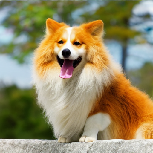
The visualizations generated by DiffusionLens illustrate a clear progression in how the model learns to associate the newly introduced token xon with the target object concept — in this case, a specific Corgi dog. As training progresses, we observe several noteworthy patterns across the text encoder layers:
Lower Layers (0–4): These layers show minimal representational change throughout training. The activations remain diffuse and unstructured, suggesting that the lower layers primarily handle syntactic or low-level token processing, without capturing high-level semantics.
Middle Layers (5–8): Here, we start to see emerging structure. The representations of
xonbegin to cluster spatially, indicating the early stages of semantic grounding. These layers act as a bridge, where the token slowly transitions from being an uninitialized placeholder to acquiring meaning aligned with the target concept.Upper Layers (9–12): The most significant transformations occur in the higher layers. By the later epochs,
xon’s activations become increasingly focused and begin to align closely with those of thedogtoken from the class prompt. Layer 12, in particular, shows a stable and semantically meaningful representation, confirming thatxonhas been successfully integrated into the learned conceptual space of “dog.”Semantic Flow: An important observation is that the concept-specific information (in this case, the Corgi dog) propagates from higher to lower layers over the course of training. While early layers remain mostly static, they begin to subtly reflect the new semantics as training progresses. This suggests that DreamBooth fine-tuning mainly affects the upper layers first, and the influence gradually trickles down the encoder.
Token Identity Transfer: Initially,
xonhas no intrinsic meaning. However, through DreamBooth fine-tuning, it learns to encapsulate the characteristics of the target reference image. The model effectively compresses the concept of the specific Corgi into thexontoken. Over time,xonbecomes semantically grounded and occupies a space in the latent representation that overlaps with the broaderdogconcept. The process demonstrates how DreamBooth builds a bridge from a personalized token to a general semantic class—storing specific visual identity inxon, and transferring it to the general “dog” representation space during generation.
2. Comparing the Raw Text Encoder vs Fine-Tuned via DreamBooth #
Objective: #
To investigate how DreamBooth fine-tuning alters the semantic understanding of special token (e.g xon) we compare the outputs of the original (pre-trained) and fine-tuned text encoder models.
Baseline Extraction:
- Use the raw text encder from
runwayml/stable-diffusion-v1-5pipeline. - Encode a promt only with specified token (e.g.,
xon) - Visualize the layer-wise embeddings.
- Use the raw text encder from
Post-Fine-Tuning Comparison:
- Repeat the same encoding process with the fine-tuned by DreamBooth approach (350 epochs) text encoder model.
- Visualize the layer-wise embeddings.
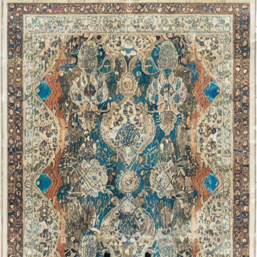
Text Encoder Layer Visualizations – Raw vs. Tuned (All Layers): #
Layer 0


Layer 1
Layer 2

Layer 3


Layer 4


Layer 5
Layer 6

Layer 7

Layer 8

Layer 9


Layer 10

Layer 11

Layer 12
Insights
We see that till up to the 10th layer, the difference in understanding the
xonconcept between the pure text encoder and the trained text encoder is not dramatic. However, beyond that point, the subsequent layers begin to retain and emphasize information specifically related to our dog.The deeper layers of the text encoder are more responsible for capturing fine-grained, learned representations associated with the fine-tuned concept.
The experiment demonstrates that DreamBooth fine-tuning impacts the deeper layers of the text encoder more significantly, encoding concept-specific details that were not present in the original model. This insight can guide future work in understanding where and how personalization occurs in diffusion model pipelines.
Note: For further details, please see our notebooks/Experiment№1_token_understanding.ipynb notebook.
3. Diving into the Latent Spaces: Understanding Representational Changes #
Objective:
The goal of this section is to explore and quantify how DreamBooth fine-tuning alters the semantic embedding of a new concept token (xon) in relation to an existing, semantically related concept (dog). We do this by probing the latent space of the CLIP text encoder, comparing the cosine similarity between the embeddings of xon and dog before and after fine-tuning.
Procedure:
We leverage the Diffusion Lens methodology to extract and compare token embeddings from both the pretrained and fine-tuned versions of the CLIP text encoder. Specifically, we:
- Tokenize a specific prompt containing the learned token
xon. - Tokenize a general prompt containing the token
dog. - Extract the embeddings corresponding to
xonanddogfrom their respective prompts. - Compute the cosine similarity between these token embeddings.
- Repeat the process for both the base encoder and the fine-tuned encoder, allowing us to quantify representational changes in the latent space.
Pseudo-code:
function compute_the_similarity(tokenizer, text_encoder, prompt_specific, prompt_general, specific_token, general_token):
    # Step 1: Tokenize both prompts
    tokens_specific = tokenizer(prompt_specific)
    tokens_general = tokenizer(prompt_general)

    # Step 2: Locate token indices in respective prompts
    index_specific = find_index(tokens_specific.input_ids, specific_token)
    index_general = find_index(tokens_general.input_ids, general_token)

    # Step 3: Encode both prompts using the provided text encoder
    embeddings_specific = text_encoder(tokens_specific)
    embeddings_general = text_encoder(tokens_general)

    # Step 4: Extract embeddings for specific tokens
    embedding_xon = embeddings_specific[index_specific]
    embedding_dog = embeddings_general[index_general]

    # Step 5: Compute cosine similarity
    similarity = cosine_similarity(embedding_xon, embedding_dog)

    return similarity
Insights:
- The cosine similarity between
xonanddogbefore fine-tuning was 0.1781, indicating low semantic alignment in the latent space of the base model. - After applying DreamBooth fine-tuning, the similarity increased to 0.2504, showing that the model has moved the representation of
xoncloser to that ofdog. - This shift suggests that DreamBooth successfully teaches the model that
xoncarries target class semantics, validating its effect on the latent space alignment of new conceptxon dog.
Note: For further details, please see our notebooks/Experiment№2_latent_representations.ipynb notebook.
Conclusion #
By combining DreamBooth fine-tuning with Diffusion Lens interpretability, we achieve not only high-fidelity, subject-driven image synthesis but also transparent insights into the model’s inner semantic processing. Our visualizations confirm that concepts emerge and sharpen progressively across text encoder and U-net layers.
References #
[1] N. Ruiz, Y. Li, V. Jampani, Y. Pritch, M. Rubinstein, and K. Aberman, Dreambooth: Fine tuning text- to-image diffusion models for subject-driven generation, 2023. arXiv: 2208.12242 [cs.CV]. [Online]. Available: https://arxiv.org/abs/2208.12242.
[2] M. Toker, H. Orgad, M. Ventura, D. Arad, and Y. Belinkov, “Diffusion lens: Interpreting text encoders in text-to-image pipelines,” Association for Computational Linguistics, 2024, pp. 9713–9728. doi: 10.18653/v1/2024.acl-long.524. [Online]. Available: http://dx.doi.org/10.18653/v1/2024.acl-long.524.