Deep Neural Decision Forests (DNDFs) with SHAP Values #
Introduction #
Deep Neural Decision Forests (DNDFs) combine the interpretability and robustness of decision trees with the power of neural networks to capture complex patterns in data. This integration allows DNDFs to perform well on various tasks, especially in high-dimensional spaces where traditional methods may struggle.
The method is different from random forests in that it uses a principled, joint, and global optimization of split and leaf node parameters and from conventional deep networks because a decision forest provides the final predictions.
Formulas Involved #
The final probability of an observation belonging to a class is the aggregated probability of that observation belonging to a class in each leaf node. The aggregation is done using a weighted sum, where the probability of the observation reaching the corresponding leaf is taken as weight. From the paper, the actual formula is as below:

Probability of an observation x belonging to class y
Learning Process #
The training of the model is done in two stages. Starting from a randomly initiated set of class probabilities for each node, iteratively update 𝜋 and µ for a predefined number of epochs.
Dataset #
Data Description: There are three types of input features:
- Objective: factual information
- Examination: results of medical examination
- Subjective: information given by the patient
Features:
- Age | int (days)
- Height | int (cm)
- Weight | float (kg)
- Gender | categorical code
- Systolic blood pressure | int
- Diastolic blood pressure | int
- Cholesterol | 1: normal, 2: above normal, 3: well above normal
- Glucose | 1, 2, 3
- Smoking | binary
- Alcohol intake | binary
- Physical activity | binary
- Presence or absence of cardiovascular disease | binary
Dataset can be found here.
Model Description #
We based our implementation on the DeepNeuralForest model available on GitHub, which is inspired by a paper on neural decision forests. We adapted the model and the training loop from this source. Specifically, we modified one of the layers in the model to better suit our dataset and added a custom class to handle our specific dataset.
The paper can be accessed here.
Model Components #
- Feature Extraction Layer: This layer is built using fully connected neural networks with ReLU activations and dropout for regularization.
- Decision Forest: This component consists of multiple decision trees, each trained on a random subset of the features.
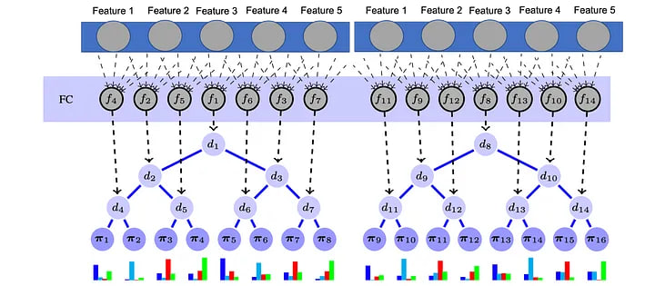
Model structure for tabular data
Implementation #
Dataset Class #
class CardioDataset(Dataset):
    """Custom dataset class for handling the cardiovascular disease dataset."""

    def __init__(self, df):
        """
        Args:
            df (pd.DataFrame): DataFrame containing the dataset.
        """
        self.data = df
        self.X = self.data.iloc[:, 1:-1].values.astype(np.float32)  # Features
        self.y = self.data.iloc[:, -1].values.astype(np.int64)      # Labels

        # Normalize the features
        self.X = (self.X - self.X.mean(axis=0)) / (self.X.std(axis=0) + 1e-6)

    def __len__(self):
        """Returns the total number of samples in the dataset."""
        return len(self.data)

    def __getitem__(self, idx):
        """
        Retrieves the feature and label for a given index.

        Args:
            idx (int): Index of the sample to retrieve.

        Returns:
            tuple: (feature, label)
        """
        return self.X[idx], self.y[idx]

def prepare_db(csv_file):
    """
    Prepares the training, validation, and test datasets.

    Args:
        csv_file (str): Path to the CSV file containing the dataset.

    Returns:
        dict: Dictionary containing the training, validation, and test datasets.
    """
    df = pd.read_csv(csv_file, sep=';')
    train_df, test_df = train_test_split(df, test_size=0.2, random_state=0)
    train_df, val_df = train_test_split(train_df, test_size=0.25, random_state=0)  # 0.25 * 0.8 = 0.2

    train_dataset = CardioDataset(train_df)
    val_dataset = CardioDataset(val_df)
    test_dataset = CardioDataset(test_df)

    return {'train': train_dataset, 'val': val_dataset, 'test': test_dataset, 'test_df': test_df}
Feature Layer #
class CardioFeatureLayer(nn.Sequential):
    """Feature extraction layer using fully connected neural networks with dropout."""

    def __init__(self, dropout_rate, shallow=False):
        """
        Args:
            dropout_rate (float): Dropout rate for regularization.
            shallow (bool, optional): Whether to use a shallow network. Defaults to False.
        """
        super(CardioFeatureLayer, self).__init__()
        self.add_module('linear1', nn.Linear(11, 1024))
        self.add_module('relu1', nn.ReLU())
        self.add_module('dropout1', nn.Dropout(dropout_rate))
        self.add_module('linear2', nn.Linear(1024, 1024))
        self.add_module('relu2', nn.ReLU())
        self.add_module('dropout2', nn.Dropout(dropout_rate))

    def get_out_feature_size(self):
        """Returns the output feature size of the layer."""
        return 1024
Tree and Forest Classes #
class Tree(nn.Module):
    """Tree class for building a single decision tree."""

    def __init__(self, depth, n_in_feature, used_feature_rate, n_class, jointly_training=True):
        """
        Args:
            depth (int): Depth of the tree.
            n_in_feature (int): Number of input features.
            used_feature_rate (float): Fraction of features to use.
            n_class (int): Number of classes.
            jointly_training (bool, optional): Whether to use joint training. Defaults to True.
        """
        super(Tree, self).__init__()
        self.depth = depth
        self.n_leaf = 2 ** depth
        self.n_class = n_class
        self.jointly_training = jointly_training

        n_used_feature = int(n_in_feature * used_feature_rate)
        onehot = np.eye(n_in_feature)
        using_idx = np.random.choice(np.arange(n_in_feature), n_used_feature, replace=False)
        self.feature_mask = onehot[using_idx].T
        self.feature_mask = Parameter(torch.from_numpy(self.feature_mask).type(torch.FloatTensor), requires_grad=False)

        if jointly_training:
            self.pi = np.random.rand(self.n_leaf, n_class)
            self.pi = Parameter(torch.from_numpy(self.pi).type(torch.FloatTensor), requires_grad=True)
        else:
            self.pi = np.ones((self.n_leaf, n_class)) / n_class
            self.pi = Parameter(torch.from_numpy(self.pi).type(torch.FloatTensor), requires_grad=False)

        self.decision = nn.Sequential(OrderedDict([
            ('linear1', nn.Linear(n_used_feature, self.n_leaf)),
            ('sigmoid', nn.Sigmoid()),
        ]))

    def forward(self, x):
        """
        Forward pass for the tree.

        Args:
            x (torch.Tensor): Input tensor.

        Returns:
            torch.Tensor: Output tensor after passing through the tree.
        """
        if x.is_cuda and not self.feature_mask.is_cuda:
            self.feature_mask = self.feature_mask.cuda()

        feats = torch.mm(x, self.feature_mask)
        decision = self.decision(feats)
        decision = torch.unsqueeze(decision, dim=2)
        decision_comp = 1 - decision
        decision = torch.cat((decision, decision_comp), dim=2)

        batch_size = x.size()[0]
        _mu = Variable(x.data.new(batch_size, 1, 1).fill_(1.))
        begin_idx = 1
        end_idx = 2
        for n_layer in range(0, self.depth):
            _mu = _mu.view(batch_size, -1, 1).repeat(1, 1, 2)
            _decision = decision[:, begin_idx:end_idx, :]
            _mu = _mu * _decision
            begin_idx = end_idx
            end_idx = begin_idx + 2 ** (n_layer + 1)

        mu = _mu.view(batch_size, self.n_leaf)
        return mu

    def get_pi(self):
        """Returns the class probabilities for the leaf nodes."""
        if self.jointly_training:
            return F.softmax(self.pi, dim=-1)
        else:
            return self.pi

    def cal_prob(self, mu, pi):
        """Calculates the probability of the input belonging to each class."""
        p = torch.mm(mu, pi)
        return p

    def update_pi(self, new_pi):
        """Updates the class probabilities for the leaf nodes."""
        self.pi.data = new_pi

class Forest(nn.Module):
    """Forest class for building a decision forest."""

    def __init__(self, n_tree, tree_depth, n_in_feature, tree_feature_rate, n_class, jointly_training):
        """
        Args:
            n_tree (int): Number of trees in the forest.
            tree_depth (int): Depth of each tree.
            n_in_feature (int): Number of input features.
            tree_feature_rate (float): Fraction of features to use for each tree.
            n_class (int): Number of classes.
            jointly_training (bool): Whether to use joint training.
        """
        super(Forest, self).__init__()
        self.trees = nn.ModuleList()
        self.n_tree = n_tree
        for _ in range(n_tree):
            tree = Tree(tree_depth, n_in_feature, tree_feature_rate, n_class, jointly_training)
            self.trees.append(tree)

    def forward(self, x):
        """
        Forward pass for the forest.

        Args:
            x (torch.Tensor): Input tensor.

        Returns:
            torch.Tensor: Output tensor after passing through the forest.
        """
        probs = []
        for tree in self.trees:
            mu = tree(x)
            p = tree.cal_prob(mu, tree.get_pi())
            probs.append(p.unsqueeze(2))
        probs = torch.cat(probs, dim=2)
        prob = torch.sum(probs, dim=2) / self.n_tree
        return prob
Neural Decision Forest Class #
class NeuralDecisionForest(nn.Module):
    """Neural Decision Forest class combining the feature extraction layer and the forest."""

    def __init__(self, feature_layer, forest):
        """
        Args:
            feature_layer (nn.Module): Feature extraction layer.
            forest (nn.Module): Decision forest.
        """
        super(NeuralDecisionForest, self).__init__()
        self.feature_layer = feature_layer
        self.forest = forest

    def forward(self, x):
        """
        Forward pass for the neural decision forest.

        Args:
            x (torch.Tensor): Input tensor.

        Returns:
            torch.Tensor: Output tensor after passing through the neural decision forest.
        """
        out = self.feature_layer(x)
        out = out.view(x.size()[0], -1)
        out = self.forest(out)
        return out
Training and Evaluation Functions #
def prepare_model(opt):
    """
    Prepares the neural decision forest model.

    Args:
        opt (dict): Dictionary containing model options.

    Returns:
        nn.Module: Neural decision forest model.
    """
    feat_layer = CardioFeatureLayer(opt['feat_dropout'])
    forest = Forest(n_tree=opt['n_tree'], tree_depth=opt['tree_depth'], n_in_feature=feat_layer.get_out_feature_size(),
                    tree_feature_rate=opt['tree_feature_rate'], n_class=opt['n_class'],
                    jointly_training=opt['jointly_training'])
    model = NeuralDecisionForest(feat_layer, forest)

    if opt['cuda']:
        model = model.cuda()
    else:
        model = model.cpu()

    return model

def prepare_optim(model, opt):
    """
    Prepares the optimizer for training.

    Args:
        model (nn.Module): Neural decision forest model.
        opt (dict): Dictionary containing optimization options.

    Returns:
        torch.optim.Optimizer: Optimizer.
    """
    params = [p for p in model.parameters() if p.requires_grad]
    return torch.optim.Adam(params, lr=opt['lr'], weight_decay=1e-5)

def train(model, optim, db, opt):
    """
    Trains the neural decision forest model.

    Args:
        model (nn.Module): Neural decision forest model.
        optim (torch.optim.Optimizer): Optimizer.
        db (dict): Dictionary containing the datasets.
        opt (dict): Dictionary containing training options.
    """
    best_val_loss = float('inf')
    for epoch in range(1, opt['epochs'] + 1):
        if not opt['jointly_training']:
            print("Epoch %d : Two Stage Learning - Update PI" % (epoch))
            cls_onehot = torch.eye(opt['n_class'])
            feat_batches = []
            target_batches = []
            train_loader = DataLoader(db['train'], batch_size=opt['batch_size'], shuffle=True)
            with torch.no_grad():
                for batch_idx, (data, target) in tqdm(enumerate(train_loader), total=len(train_loader), desc="Updating PI"):
                    if opt['cuda']:
                        data, target, cls_onehot = data.cuda(), target.cuda(), cls_onehot.cuda()
                    data = Variable(data)
                    feats = model.feature_layer(data)
                    feats = feats.view(feats.size()[0], -1)
                    feat_batches.append(feats)
                    target_batches.append(cls_onehot[target])

                for tree in model.forest.trees:
                    mu_batches = []
                    for feats in feat_batches:
                        mu = tree(feats)
                        mu_batches.append(mu)
                    for _ in range(20):
                        new_pi = torch.zeros((tree.n_leaf, tree.n_class))
                        if opt['cuda']:
                            new_pi = new_pi.cuda()
                        for mu, target in zip(mu_batches, target_batches):
                            pi = tree.get_pi()
                            prob = tree.cal_prob(mu, pi)
                            pi = pi.data
                            prob = prob.data
                            mu = mu.data
                            _target = target.unsqueeze(1)
                            _pi = pi.unsqueeze(0)
                            _mu = mu.unsqueeze(2)
                            _prob = torch.clamp(prob.unsqueeze(1), min=1e-6, max=1.)
                            _new_pi = torch.mul(torch.mul(_target, _pi), _mu) / _prob
                            new_pi += torch.sum(_new_pi, dim=0)
                        new_pi = F.softmax(Variable(new_pi), dim=1).data
                        tree.update_pi(new_pi)

        model.train()
        train_loader = DataLoader(db['train'], batch_size=opt['batch_size'], shuffle=True)
        running_loss = 0.0
        correct = 0
        total = 0
        with tqdm(total=len(train_loader), desc=f'Epoch {epoch}') as pbar:
            for batch_idx, (data, target) in enumerate(train_loader):
                if opt['cuda']:
                    data, target = data.cuda(), target.cuda()
                data, target = Variable(data), Variable(target)
                optim.zero_grad()
                output = model(data)
                loss = F.nll_loss(torch.log(output + 1e-6), target)  # Add small epsilon to prevent NaNs
                loss.backward()
                optim.step()

                running_loss += loss.item()
                pred = output.data.max(1, keepdim=True)[1]
                correct += pred.eq(target.data.view_as(pred)).cpu().sum().item()
                total += target.size(0)

                pbar.set_postfix({'loss': running_loss / (batch_idx + 1), 'accuracy': correct / total})
                pbar.update(1)

        val_loss, val_accuracy = evaluate(model, db['val'], opt, desc="Validating")
        print(f'\nValidation set: Average loss: {val_loss:.4f}, Accuracy: {val_accuracy:.4f}\n')

        # Log metrics to wandb
        wandb.log({
            'epoch': epoch,
            'train_loss': running_loss / len(train_loader),
            'train_accuracy': 100. * correct / total,
            'val_loss': val_loss,
            'val_accuracy': val_accuracy
        })

        # Save the best model
        if val_loss < best_val_loss:
            best_val_loss = val_loss
            torch.save(model.state_dict(), 'best_model_7.pth')

    # Load the best model and make predictions on the test set
    model.load_state_dict(torch.load('best_model_7.pth'))
    test_loss, test_accuracy = evaluate(model, db['test'], opt, desc="Testing")
    print(f'\nTest set: Average loss: {test_loss:.4f}, Accuracy: {test_accuracy:.4f}\n')

    # Log test metrics to wandb
    wandb.log({
        'test_loss': test_loss,
        'test_accuracy': test_accuracy
    })

    # Predict on the test set and print results
    predictions = predict(model, db['test'], opt)
    print(f'Test set predictions:\n {predictions}')

    # SHAP explanations
    shap_explainer(model, db['test_df'], opt)
Evaluation and Prediction Functions #
def evaluate(model, dataset, opt, desc="Evaluating"):
    """
    Evaluates the model on the given dataset.

    Args:
        model (nn.Module): Neural decision forest model.
        dataset (Dataset): Dataset to evaluate on.
        opt (dict): Dictionary containing evaluation options.
        desc (str): Description for the progress bar.

    Returns:
        tuple: (average loss, accuracy)
    """
    model.eval()
    loader = DataLoader(dataset, batch_size=opt['batch_size'], shuffle=False)
    test_loss = 0
    correct = 0
    with tqdm(total=len(loader), desc=desc) as pbar:
        with torch.no_grad():
            for data, target in loader:
                if opt['cuda']:
                    data, target = data.cuda(), target.cuda()
                data, target = Variable(data), Variable(target)
                output = model(data)
                test_loss += F.nll_loss(torch.log(output + 1e-6), target, reduction='sum').item()  # Add small epsilon to prevent NaNs
                pred = output.data.max(1, keepdim=True)[1]
                correct += pred.eq(target.data.view_as(pred)).cpu().sum().item()
                pbar.set_postfix({'val_loss': test_loss / len(loader.dataset), 'val_accuracy': correct / len(loader.dataset)})
                pbar.update(1)

    test_loss /= len(loader.dataset)
    accuracy = correct / len(loader.dataset)
    return test_loss, accuracy

def predict(model, dataset, opt):
    """
    Predicts the class labels for the given dataset.

    Args:
        model (nn.Module): Neural decision forest model.
        dataset (Dataset): Dataset to predict on.
        opt (dict): Dictionary containing prediction options.

    Returns:
        list: List of predicted class labels.
    """
    model.eval()
    loader = DataLoader(dataset, batch_size=opt['batch_size'], shuffle=False)
    predictions = []
    with torch.no_grad():
        for data, _ in loader:
            if opt['cuda']:
                data = data.cuda()
            data = Variable(data)
            output = model(data)
            pred = output.data.max(1, keepdim=True)[1]
            predictions.extend(pred.cpu().numpy().flatten())
    return predictions
SHAP Explanations #
def shap_explainer(model, dataset, opt):
    """
    Generates SHAP explanations for the model predictions.

    Args:
        model (nn.Module): Neural decision forest model.
        dataset (dict): Dictionary containing the test dataset.
        opt (dict): Dictionary containing SHAP options.
    """
    def model_predict(data):
        return np.array(predict(model, data, opt))

    X_test = dataset["test"].X  # Use the dataset's features for SHAP values

    X_sample = X_test[np.random.randint(0, len(X_test), 100)]

    explainer = shap.KernelExplainer(model_predict, X_sample)
    shap_values = explainer.shap_values(X_sample, nsamples=100)

    # Plot the summary plot
    shap.summary_plot(shap_values, X_sample, plot_type="bar",
                      feature_names=['age', 'gender', 'height', 'weight', 'ap_hi', 'ap_lo', 'cholesterol', 'gluc', 'smoke', 'alco', 'active'])

    shap.summary_plot(shap_values, features=X_sample, class_inds=[1], max_display=10,
                      feature_names=['age', 'gender', 'height', 'weight', 'ap_hi', 'ap_lo', 'cholesterol', 'gluc', 'smoke', 'alco', 'active'])
Main Function #
def main():
    """
    Main function to initialize wandb, prepare data, model, optimizer, and start training.
    """
    wandb.init(project="cardio_prediction", config={
        'batch_size': 128,
        'feat_dropout': 0.3,
        'n_tree': 5,
        'tree_depth': 3,
        'n_class': 2,
        'tree_feature_rate': 0.5,
        'lr': 0.001,
        'gpuid': -1,
        'jointly_training': False,
        'epochs': 20,
        'report_every': 10
    })
    config = wandb.config

    # Manually define arguments
    opt = {
        'batch_size': config.batch_size,
        'feat_dropout': config.feat_dropout,
        'n_tree': config.n_tree,
        'tree_depth': config.tree_depth,
        'n_class': config.n_class,
        'tree_feature_rate': config.tree_feature_rate,
        'lr': config.lr,
        'gpuid': config.gpuid,
        'jointly_training': config.jointly_training,
        'epochs': config.epochs,
        'report_every': config.report_every,
        'cuda': torch.cuda.is_available()
    }

    if opt['gpuid'] >= 0:
        torch.cuda.set_device(opt['gpuid'])
    else:
        print("WARNING: RUN WITHOUT GPU")

    db = prepare_db('cardio_train.csv')
    model = prepare_model(opt)
    optim = prepare_optim(model, opt)
    train(model, optim, db, opt)

if __name__ == '__main__':
    main()
Results #
Model Performance #
The model demonstrated a steady improvement in training accuracy, reaching approximately 74% by the 20th epoch. Validation accuracy showed a similar trend, indicating that the model was effectively learning from the training data without overfitting.
Training Accuracy #
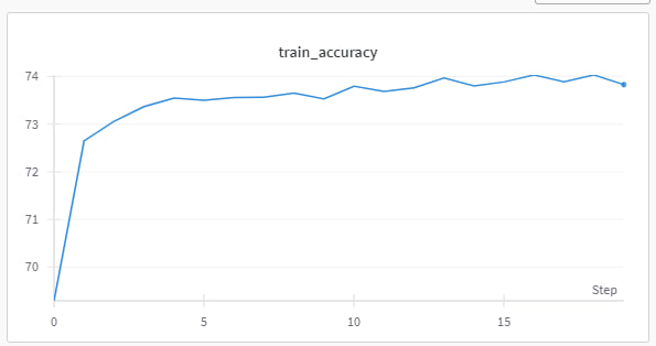
Training Accuracy
Training and Validation Metrics #

Validation Accuracy, Training Loss, Validation Loss
SHAP Values #
Tree SHAP is an algorithm used to compute exact SHAP values for Decision Tree-based models. SHAP (SHapley Additive exPlanation) is a game-theoretic approach to explain the output of any machine learning model. The goal of SHAP is to explain the prediction for any instance ( x_i ) as a sum of contributions from its individual feature values.
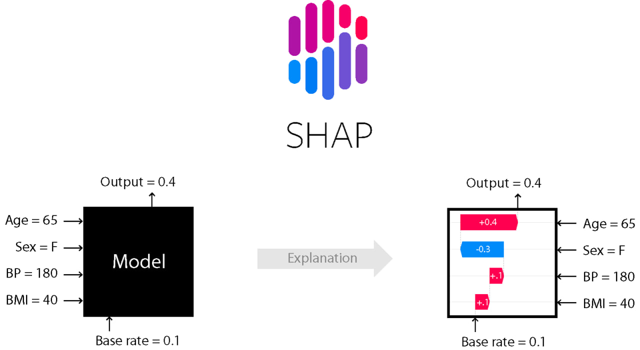
As explained in the first article, SHAP values are obtained from the following equation:
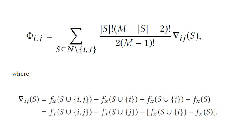
SHAP Equation
This method is part of the additive feature attribution methods class; feature attribution refers to the fact that the change of an outcome to be explained (e.g., a class probability in a classification problem) with respect to a baseline (e.g., average prediction probability for that class in the training set) can be attributed in different proportions to the model input features.
SHAP Interaction Values #
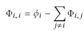
SHAP allows us to compute interaction effects by considering pairwise feature attributions. This leads to a matrix of attribution values representing the impact of all pairs of features on a given model prediction. SHAP interaction effect is based on the Shapley interaction index from game theory and is given by:
SHAP Interaction Values
The above equation indicates that the SHAP interaction value of the ( i )-th feature with respect to the ( j )-th feature can be interpreted as the difference between SHAP values of the ( i )-th feature with and without the ( j )-th feature. This allows us to use the algorithm for computing SHAP values to compute SHAP interaction values.
Challenges #
Training on a real dataset presented several additional challenges:
- Computational Resources: Training the model on a larger real-world dataset required substantial computational resources. Efficient use of GPU acceleration and parallel processing was necessary to manage training times.
- SHAP Integration: Integrating SHAP for model explainability was challenging due to the custom architecture of the neural decision forest. Ensuring compatibility and efficient computation of SHAP values required careful handling.
Insights from SHAP #
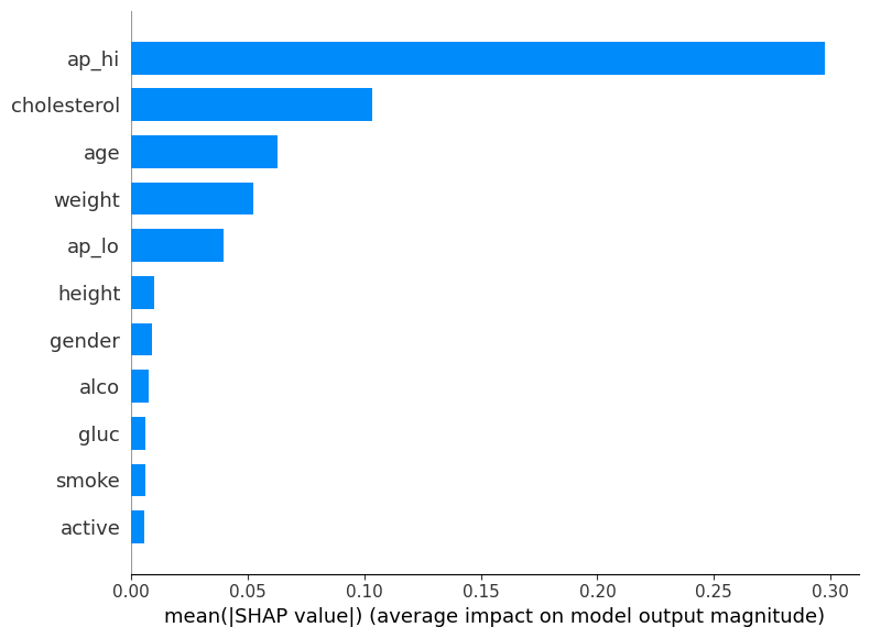
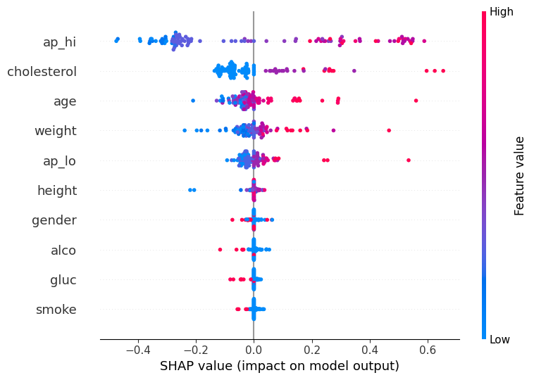
The integration of SHAP provided valuable insights into the model’s predictions. The SHAP summary plot highlighted the most influential features in the model’s decision-making process.
From the plot, we can observe that the top features impacting the model’s predictions are:
- Systolic Blood Pressure (ap_hi)
- Cholesterol Levels
- Age
- Weight
- Diastolic Blood Pressure (ap_lo)
These features have the highest mean absolute SHAP values, indicating their significant influence on the prediction of cardiovascular disease.
SHAP Summary Plot #
SHAP Summary Plot
SHAP Beeswarm Plot #
SHAP Beeswarm Plot
Conclusion #
Deep Neural Decision Forests offer a powerful combination of decision trees and neural networks, providing both high performance and interpretability. The addition of SHAP values further enhances the model’s transparency, making it easier to understand and trust the predictions.
For those interested in further exploration, the full implementation is provided, including the training process and SHAP integration for interpretability.
Happy coding!