Building Explainable Hiring Models with CatBoost and SHAP #
Authors: Amir Nigmatullin ( am.nigmatullin@innopolis.university) and Nurislam Zinnatullin ( n.zinnatullin@innopolis.university)
1. Introduction #
Explainable Artificial Intelligence (XAI) has become a fundamental area of AI research, striving to improve the transparency and interpretability of machine learning models. Understanding how AI systems make decisions is crucial for fostering trust, ensuring accountability, and mitigating potential risks.
In this post, we focus on the application of AI in hiring decisions, where biased models can lead to significant legal and ethical challenges, as well as financial losses in the future. By leveraging the expertise of HR specialists, we can train a model that aligns with their decision-making processes. To enhance interpretability, we propose using SHAP (Shapley Additive Explanations) to estimate the factors influencing predictions. Specifically, we will explore the use of the CatBoost classifier to ensure accurate and explainable hiring decisions
2. CatBoost: Architecture and Advantages #
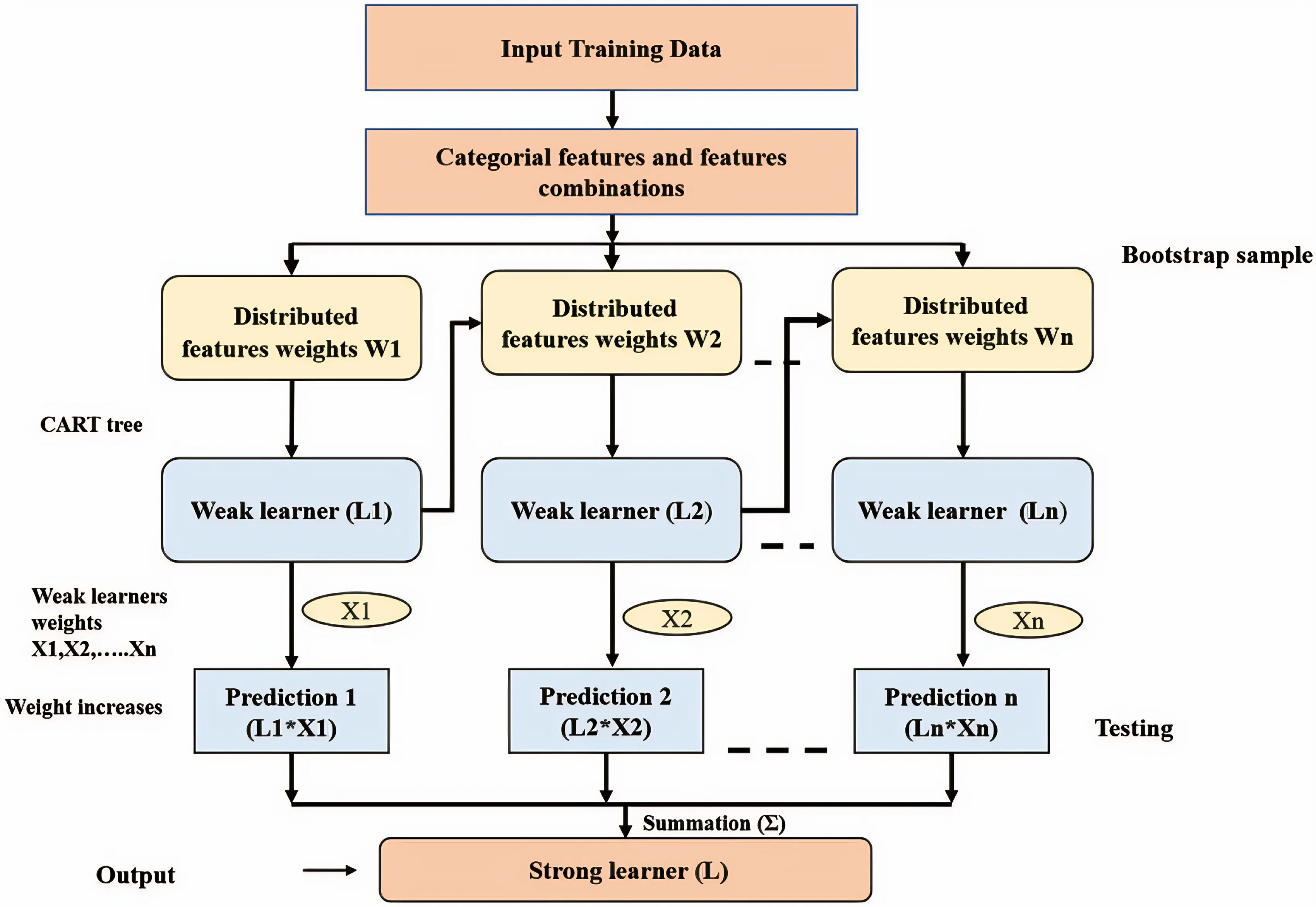
CatBoost, a state-of-the-art algorithm developed by Yandex, is a powerful solution for efficient and accurate machine learning tasks, including classification and regression. With its innovative Ordered Boosting technique, CatBoost enhances predictive performance by leveraging decision trees effectively.
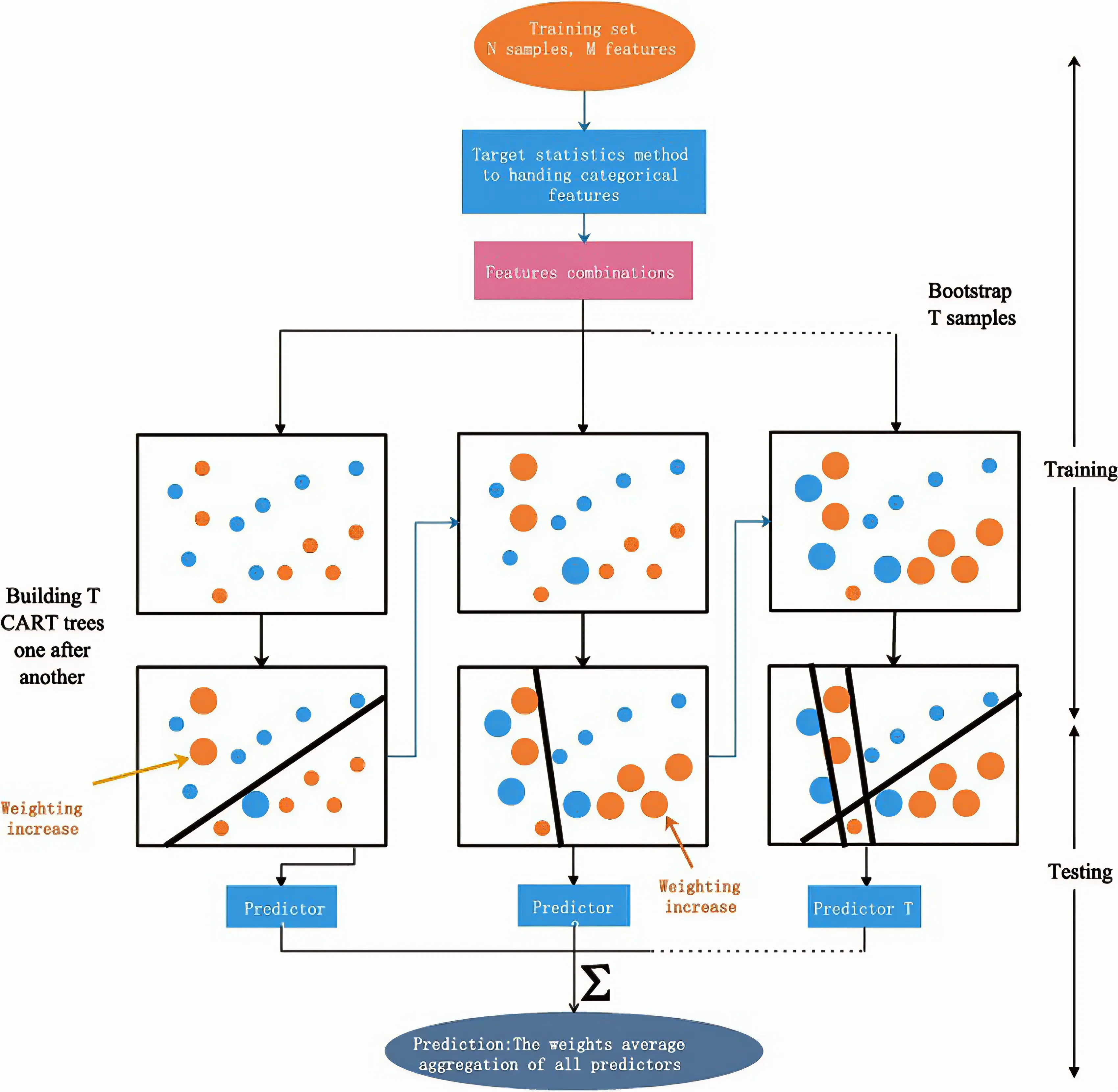
A major advantage of CatBoost is its efficient handling of categorical features. It utilizes a unique approach known as “ordered boosting,” which enables the model to process categorical data directly. This method enhances training speed and boosts model accuracy by encoding categorical variables while maintaining their inherent order.
Our dataset mainly consisted of categorical or near-categorical features (Age, Gender, EducationLevel, ExperienceYears, InterviewScore, SkillScore, PersonalityScore, RecruitmentStrategy), therefore we decided to choose CatBoost as a recruitment system model.
3. Understanding SHAP and Shapley Values #
SHAP is a state-of-the-art method that explains model predictions by quantifying the contribution of each feature. Its foundation lies in Shapley values from cooperative game theory.
Shapley Values from Game Theory #
Originally proposed by Lloyd Shapley in 1953, Shapley values were designed to fairly distribute a total payoff among players in a cooperative game. In our context:
- Players: The features of the model.
- Payoff: The prediction outcome.
The Shapley value for a feature i is calculated as:
\[\phi_i = \sum_{S \subseteq N \setminus \{i\}} \frac{|S|! (|N| - |S| - 1)!}{|N|!} \left[ f(S \cup \{i\}) - f(S) \right]\]Where:
- N is the set of all features.
- S is any subset excluding feature i.
- f(S) is the model prediction using subset S.
- The factorial terms account for all possible inclusion orders.
A Simple Example
Suppose your model uses 3 features: Age, Income, and Education. To compute the Shapley value for “Income”, we look at every possible way to add “Income” into different combinations of the other features and see how much the prediction changes when we do that.
We repeat this for all combinations and average the effect. This way, even if “Income” interacts with “Education”, its impact is fairly shared.
SHAP in Machine Learning #
SHAP leverages these values to provide explanations for individual predictions as well as overall model behavior. Its key properties include:
- Additivity:
Model predictions can be decomposed as a sum of a baseline value \(\phi_0\) and individual SHAP values \(\phi_i\) :
For example, in ensemble models like random forests Additivity property guarantees that for a feature value, you can calculate the Shapley value for each tree individually, average them, and get the Shapley value for the feature value for the random forest.
Fairness:
Features with similar contributions receive similar SHAP values.Zero Importance:
Features that do not affect the prediction have SHAP values close to zero.
4. Efficient Approximation of Shapley Values #
Calculating exact Shapley values is computationally expensive due to the need to evaluate all possible subsets of features (exponential in number). To overcome this, approximation methods are used.
Kernel SHAP (KernelExplainer) #
Kernel SHAP approximates Shapley values via weighted linear regression on a subset of feature coalitions.
How It Works:
- Coalition Sampling:
Instead of evaluating all (2^M) subsets (M is number of features), it samples a limited number (using a parameter likemax_samples) with weights determined by the Shapley kernel:
This prioritizes small (1-2 features) and large (M-1 to M-2 features) coalitions, which carry the highest information value.
Background Data Integration:
For each coalition, creates masked instances by blending the target observation’s features withbackground_data(typically 10-100 samples). Predictions on these hybrid instances approximate f(S ⋃ i) and f(S).Regression:
Uses weighted linear regression to solve for Shapley values that best explain the prediction differences:
This reduces the complexity from O(2^M) to O(S · P + M^3), where
- M is number of features
- S is number of sampled coalitions in Kernel SHAP
- B is number of background samples in SamplingExplainer
- P is cost of a single model prediction (e.g., one forward pass)
- Model evaluations: O(S⋅P) because we sample S coalitions and evaluate the model once per coalition
- Regression fit: O((M+1)^3) to solve the weighted linear system for M feature weights plus the intercept.
Pseudo-code #
Input:
  f         := trained model
  x         := target instance (length-M vector)
  D         := background dataset {z₁…z_B}
  S         := number of coalitions to sample

Output:
  φ₁…φ_M    := SHAP values (no φ₀; can be reconstructed from expected value)

1.  Sample background indices D′ ⊆ D
2.  Generate S coalitions C₁…C_S where each C_j ⊆ {1…M}

3.  For each j = 1…S:
4.    Compute kernel weight:
        w_j ← (M−1) / (|C_j| · (M−|C_j|))    ⟶ Shapley kernel

5.    For each z ∈ D′:
6.      Create masked sample x^{(j)}_z:
         [x^{(j)}_z]_i = x_i   if i ∈ C_j
                        z_i   otherwise

7.    Compute y_j ← (1/B) * Σ_{z∈D′} f(x^{(j)}_z)

8.  End for

9.  Use weighted linear regression:
       Fit φ minimizing Σ_j w_j · (y_j − (Σ_{i∈C_j} φ_i))²

10. Return φ₁…φ_M
Sampling-Based Approximation (SamplingExplainer) #
SamplingExplainer uses feature perturbation and averaging over background data to estimate feature contributions more quickly.
Key Steps:
Baseline Prediction:
Compute average predictions using background data.Perturbation Analysis:
For each feature in the target instance:- Replace the feature’s value in all background samples with the instance’s value
- Compute prediction deltas in log-odds space
- Average deltas across background samples as the feature’s contribution
Additivity Enforcement:
\[ \sum\phi_i = f(x) - E[f] \]
Rescales contributions to ensure:
This preserves SHAP’s local accuracy guarantee.
Complexity scales as O(B·M·P) where B is background samples (typically 100-1000) and others you can see in kernel SHAP section.
Pseudo-code #
Input:
  f       := trained model
  x       := target instance (length-M vector)
  D       := background dataset {z₁…z_B}
  L       := background predictions in log-odds space

Output:
  φ₀…φ_M  := SHAP values (including intercept φ₀)

1.  Compute log-odds baseline:
      φ₀ ← (1/B) * Σ_{z∈D} logit(f(z))       ⟶ baseline in log-odds space

2.  Compute log-odds of f(x):
      logit_f_x ← logit(f(x))

3.  For each feature i = 1…M:
4.    For each background point z ∈ D:
5.      Create z^{(i)} where
         [z^{(i)}]_i = x_i
         [z^{(i)}]_k = z_k    for k ≠ i
6.      Compute δ_{i,z} ← logit(f(z^{(i)})) − logit(f(z))
7.    End for
8.    φ_i ← (1/B) * Σ_{z∈D} δ_{i,z}
9.  End for

10. Enforce additivity:
      total ← Σ_{i=1}^M φ_i
      adjust ← logit_f_x − φ₀ − total
      Distribute `adjust` proportionally or add to φ₁

11. Return φ₀…φ_M
Sampling strategy #
A sampling strategy is simply a way to pick a manageable number of examples instead of checking every possible case. In our SHAP implementation, we used two such strategies:
Kernel SHAP: we randomly choose groups of features—giving priority to very small and very large groups—to see how including them changes the model’s output.
SamplingExplainer: we randomly draw past data points and swap in one feature at a time from the instance we’re explaining, measuring how each swap shifts the prediction.
These methods let us approximate each feature’s contribution quickly and accurately without testing all possible feature combinations.
Tradeoffs and Practical Considerations #
| Method | Strength | Limitation |
|---|---|---|
| KernelExplainer | Theoretically robust, model-agnostic | Slower for high M, sensitive to S |
| SamplingExplainer | Very simple, scales linearly in M | Assumes feature independence |
5. Our Recruitment Model: Case Study #
We applied our approach to build an autonomous hiring system using historical HR data. Our model is based on CatBoost, chosen for its excellence in handling categorical data.
Model Performance Metrics #
Accuracy:
 0.9566666666666667

ROC AUC Score:
 0.941313269493844

Classification Report:
               precision    recall  f1-score   support

           0       0.96      0.98      0.97       215
           1       0.94      0.91      0.92        85

    accuracy                           0.96       300
   macro avg       0.95      0.94      0.95       300
weighted avg       0.96      0.96      0.96       300
Feature Analysis #
While our EDA we found key predictors that were highly correlated with hiring decisions:
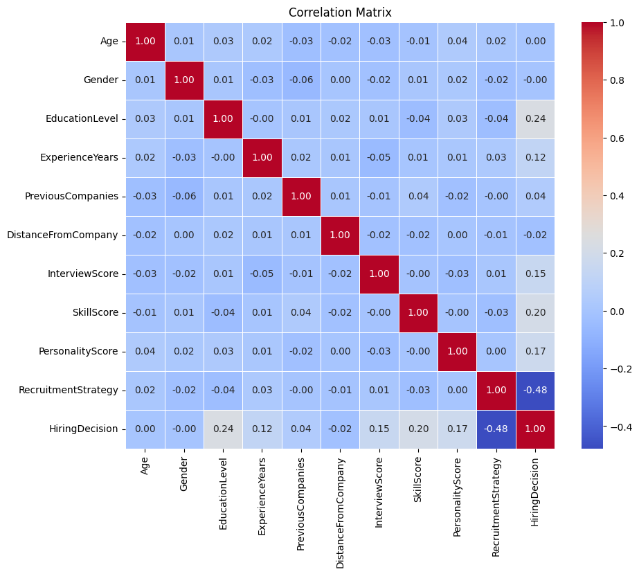
RecruitmentStrategy, EducationLevel, SkillScore, PersonalityScore, and ExperienceYears
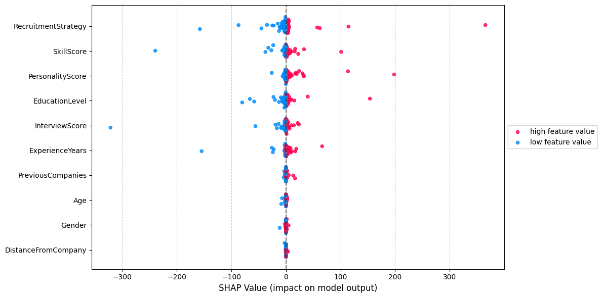
Beeswarm plot: #
A SHAP beeswarm plot visualizes the distribution and impact of each feature’s SHAP values across all predictions, showing feature importance (vertical order) and effect direction (red/blue for positive/negative influence). It helps identify key drivers of model behavior while revealing nonlinear patterns and outliers in feature contributions.
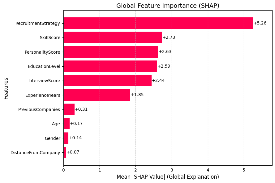
Bar plot (Global): #
The SHAP bar plot ranks features by their average impact (mean absolute SHAP values), showing which features most influence the model’s predictions across all data.
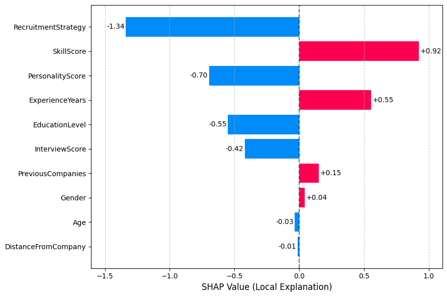
Bar plot (Local): #
For a single prediction, it displays each feature’s exact contribution (positive/negative SHAP value), explaining how they pushed the prediction higher or lower than the baseline. This can help HR specialists understand why a specific candidate was recommended or not.
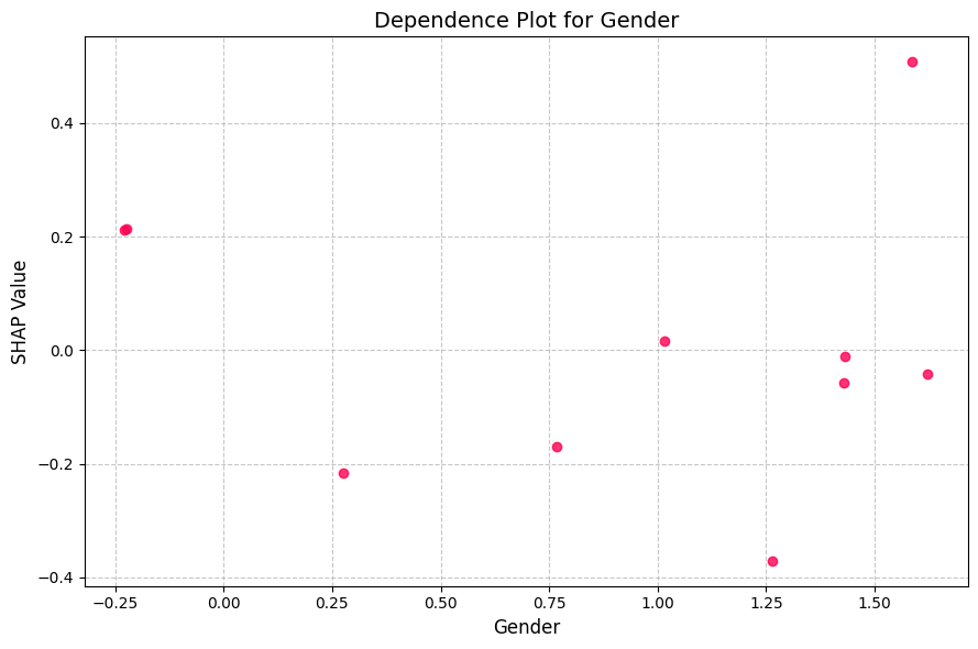
Dependence plot: #
The dependence plot shows how the impact of feature varies across different values, revealing non-linear relationships not captured by simple correlation
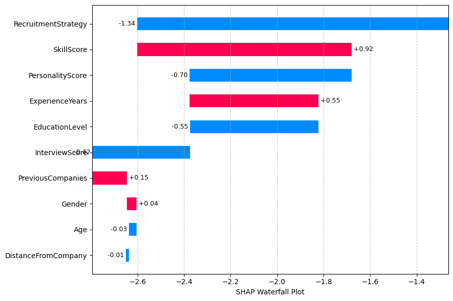
Waterfall plot: #
The waterfall plot for a specific candidate shows how each feature contributed to their final prediction, providing transparency for individual decisions
Built-in Feature importance by CatBoost #
Visual plots from both SHAP approaches and the built-in CatBoost feature importance revealed consistent insights, aligning well with our initial exploratory data analysis.
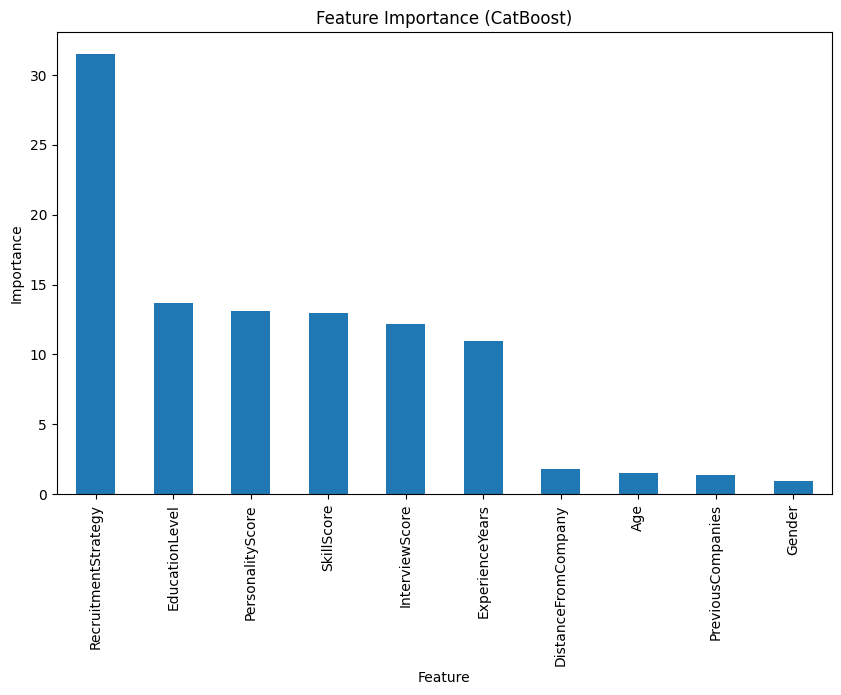
Why not use only CatBoost feature importance? #
It shows average magnitude of feature impact across the dataset
SHAP values provide detailed feature contributions for each prediction, showing both magnitude and direction. So it can interpret not only global features importance, but also individual instance interpretation.
6. Key Insights and Recommendations #
Insights #
Strategic Hiring:
Aggressive recruitment strategies can significantly influence hiring outcomes.Candidate Evaluation:
Educational background and technical skills are strong predictors.Fairness:
The model shows minimal bias based on demographic features like age and gender.Transparency:
XAI techniques such as SHAP enhance trust by explaining the model’s predictions both globally and locally.
Recommendations for Business #
- Adjust Recruitment Strategies:
Align strategies with market conditions and organizational needs. - Focus on Predictive Factors:
Prioritize education and skills in candidate evaluation. - Continuous Monitoring:
Regularly audit the model using SHAP to maintain fairness and accuracy. - Embrace Interpretability:
Incorporate explainability into all high-stakes decision-making systems to ensure transparency and accountability.
7. Conclusion #
By integrating CatBoost and SHAP, we not only achieve high model performance but also offer deep insights into the decision-making process. This dual focus on accuracy and interpretability supports fair and informed HR practices, making it a powerful approach for modern recruitment systems.
8. References #
Dataset that we used to train the hiring model
Original article about SHAP values