Fair Sentencing: An Explainable and Fair Approach to Predicting Court Decisions #
Introduction #
The American correction system struggles with lack of resources to contain prisoners and mentally ill people. To prevent correction system’s overflow, modern courts use different assessments algorithms - including risk prediction software made by Northpointe that was criticised in by ProPublica [1]. Authors of the article collected statistical information of the model’s results and concluded that it is biased against black people. There is no information how the model actually work - it is assumed as “intellectual property” of the company. However, the authors of ProPublica can also be biased: “One tool being used in states including Kentucky and Arizona, called the Public Safety Assessment, was developed by the Laura and John Arnold Foundation, which also is a funder of ProPublica”. So, I decided to check if the model is actually biased and, if it is biased, why so.


Random Forest Regressor (RFR) #
Conceptual Foundation #
Random Forest is an ensemble learning method that operates by constructing multiple decision trees during training and outputting the mean prediction of individual trees. For regression tasks, it provides:
- Robustness through variance reduction via bagging
- Non-linearity inherent in decision tree structures
- Feature importance metrics for interpretability
Mathematical Formulation #
The ensemble prediction combines T regression trees:
\[ \hat{y}(x) = \frac{1}{T}\sum_{t=1}^T f_t(x) \]Where:
- \(t\) - t-th tree
- \(T\) - total number of trees
- \(f_t\) = prediction of the t-th decision tree
- \(x\) = parameters of t-th tree
- Each tree predicts independently on a bootstrap sample
Implementation Details #
Key components in my custom implementation:
class DecisionTreeRegressor:
    def _build_tree(self, X, y, depth=0):
        # Stopping conditions:
        # 1. Reached max depth
        # 2. Not enough samples to split
        # 3. All target values are identical
        if (depth == self.max_depth or
                len(y) < self.min_samples_split or
                len(np.unique(y)) == 1):
            return self.Node(value=np.mean(y))  # Create leaf node

        feature, threshold = self._best_split(X, y)
        if feature is None:  # No improvement possible
            return self.Node(value=np.mean(y))

        # Recursively build left and right subtrees
        left_idx = X[:, feature] <= threshold
        left = self._build_tree(X[left_idx], y[left_idx], depth + 1)
        right = self._build_tree(X[~left_idx], y[~left_idx], depth + 1)

        return self.Node(feature, threshold, left, right)
Advantages of Random Forest Regressor in this project #
| advantage | description |
|---|---|
| Handles mixed data types | Accommodates both categorical (race, gender) and numerical (age, priors) features |
| Feature importance | Identifies racial bias through explicit importance scores |
| Robust to outliers | Mitigates impact of extreme criminal histories |
Limitations #
- Black box: While feature importance is provided, exact decision paths remain opaque
- Correlated features: May over-prioritize demographic variables due to correlations with criminal history
- Data dependence: Inherits biases present in training data
Fairness-Aware Counterfactual Explanations (FACE) #
Conceptual Foundation: #
FACE generates scenarios “WHAT-IF” scenarios that:
- Identify minimal changes to input features
- Achieve desired model output
- Respect fairness constraints (can immute features)
Mathematical background: #
The counterfactual search solves: \[ \underset{x'}{\text{min}} \underbrace{(f(x') - y_t)^2}_{\text{Target}} + \lambda \underbrace{\sum_{i \notin \mathcal{I}} (x'_i - x_i)^2}_{\text{Proximity}} \]
Where:
- \(x'\) is the counterfactual instance
- \(f\) is the model’s prediction function
- \(y_t\) is the target prediction score
- \(\mathcal{I}\) is the set of immutable feature indices
- \(\lambda\) controls the trade-off between objectives
Implementation #
Custom FACE generator:
def generate_face(rf_model, x_orig, y_target, feature_names, immutable_features=[], lambda_=0.5, max_iter=1000, tol=0.1):
  # Convert input to numpy array
  x_orig = np.array(x_orig).astype(float) if not isinstance(x_orig, np.ndarray) else x_orig.copy()
  x_cf = x_orig.copy()

  # Create immutable mask
  immutable_mask = np.array([f in immutable_features for f in feature_names], dtype=bool)

  # Optimization loop
  for _ in range(max_iter):
    # Current prediction and residual
    y_pred = rf_model.predict(x_cf.reshape(1, -1))[0]
    residual = y_pred - y_target

    # Check convergence
    if abs(residual) < tol:
      break

    # Numerical gradient computation
    grad = np.zeros_like(x_cf)
    eps = 1e-5  # Smaller epsilon for better gradient approximation

    for i in range(len(x_cf)):
      if immutable_mask[i]:
        continue

      # Perturb feature
      x_temp = x_cf.copy()
      x_temp[i] += eps

      # Get directional derivative
      y_temp = rf_model.predict(x_temp.reshape(1, -1))[0]
      model_derivative = (y_temp - y_pred) / eps

      # Complete gradient term (2r*df/dx + 2λ(x'-x))
      grad[i] = 2 * residual * model_derivative + 2 * lambda_ * (x_cf[i] - x_orig[i])

    # Projected gradient update
    learning_rate = 0.01  # Can be made adaptive
    x_cf -= learning_rate * grad

    # Enforce immutability and bounds
    x_cf[immutable_mask] = x_orig[immutable_mask]
    x_cf = np.clip(x_cf, 0, 1)  # Assuming normalized features

  return x_cf
Advantages for Bias Analysis #
| advantage | description |
|---|---|
| Actionable recourse | Shows how defendants could improve scores |
| Immutable constraints | Isolates discriminatory features by locking race/gender |
| Quantitative comparison | Measures disparity in effort required across demographics |
Limitations #
- Computational intensity: Requires multiple model evaluations per sample
- Discrete features: Challenges in handling categorical variables (e.g. races)
- Local explanations: May miss systemic patterns visible only in global analysis
Method selection explanation #
Why Random Forest Regression: #
- Handles COMPAS data characteristics:
- Mixed feature types (categorical + numerical)
- Non-linear relationships between features and score
- Provides interpretability tools:
- Feature importance scores
- Partial dependence plots
- SHAP value compatibility
- Robust performance with minimal hyperparameter tuning
Why FACE: #
- Directly tests fairness by:
- Quantifying racial bias through immutable feature locking
- Measuring disparity in required changes across groups
- Provides actionable insights beyond typical fairness metrics:
print(f"Score reduction for Caucasian: {face_caucasian.changes}")
print(f"Score reduction for African-American: {face_aa.changes}")
- Show easily interpreted data:
Before we start #
Let us just check the basic statistics:
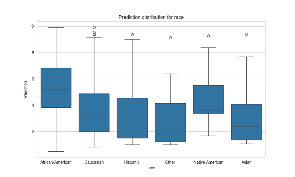
The model really seems biased to races, especially African-Americans and Native Americans
Results #
Random Forest Regressor: #
After initialization and training, let us check the importance of different features for the model:
| feature | importance |
|---|---|
| num__age | 0.447778 |
| num__priors_count | 0.446711 |
| cat__race_African-American | 0.050874 |
| num__juv_fel_count | 0.013764 |
| cat__c_charge_degree_M | 0.011301 |
| cat__race_Caucasian | 0.006735 |
| num__juv_misd_count | 0.004238 |
| cat__c_charge_degree_O | 0.004137 |
| cat__race_Other | 0.003599 |
| cat__sex_Male | 0.003294 |
And here is interesting things happening: age of the person is the most important parameter (even more, than number of prior crimes), and African-American race has more impact than Felony crimes commited in minor! Let us just leave it here and discuss later.
FACE: #
Then, we take random sample that taken COMPAS score higher, than 7. That sample is 24 y.o. African-American male with 0 priors before and no crimes in minor. Let us apply FACE to this sample with ‘age’ chosen as immutable parameter. The result is ridiculous:
| Features transformed |
|---|
| num__priors_count: -0.660 → -3.174 |
| cat__race_Asian: 0.000 → 1.176 |
| cat__race_Caucasian: 0.000 → 0.783 |
| cat__race_Hispanic: 0.000 → 0.521 |
| cat__race_Native American: 0.000 → -0.531 |
| cat__race_Other: 0.000 → 1.914 |
| cat__c_charge_degree_M: 0.000 → 0.514 |
To reduce the score, model “suggest” at most to decrease number of priors (which is 0 already!) and change the race of a person. Moreover, race has impact more, than degree of the current charge.
Well, let’s try to apply FACE again, but now lock everything except ‘race’:
| Features transformed |
|---|
| cat__race_Asian: 0.000 → 1.176 |
| cat__race_Caucasian: 0.000 → 0.783 |
| cat__race_Hispanic: 0.000 → -0.527 |
| cat__race_Native American: 0.000 → -1.050 |
| cat__race_Other: 0.000 → 1.914 |
And again, model shows high discrimination for some races and aggregation for others.
Next, let us check FACE on two samples, which differ only in race:
For African-American:
| Features transformed |
|---|
| num__age: 1.415 → 1.533 |
| num__priors_count: -0.232 → -3.196 |
| cat__c_charge_degree_M: 0.000 → 0.683 |
| cat__c_charge_degree_O: 0.000 → -0.778 |
For Caucasian:
| Features transformed |
|---|
| num__age: 1.415 → 2.681 |
| num__priors_count: -0.232 → -1.631 |
| cat__c_charge_degree_M: 0.000 → 1.433 |
| cat__c_charge_degree_O: 0.000 → 0.096 |
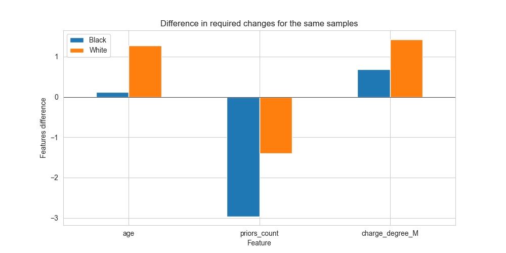
As we can see, for the same person the model suggests different method of reducing COMPAS score: while for Caucasians it is enough just to change age or degree, for African-Americans previous crimes are crucial. That is means, that for aged white people the model significantly decrease the score, while for African-Americans - no.
Analysis #
To understand, why model has such strange bias, we need to check different statistics provided.
SHAP: #
Use SHAP to check how features impact on result:
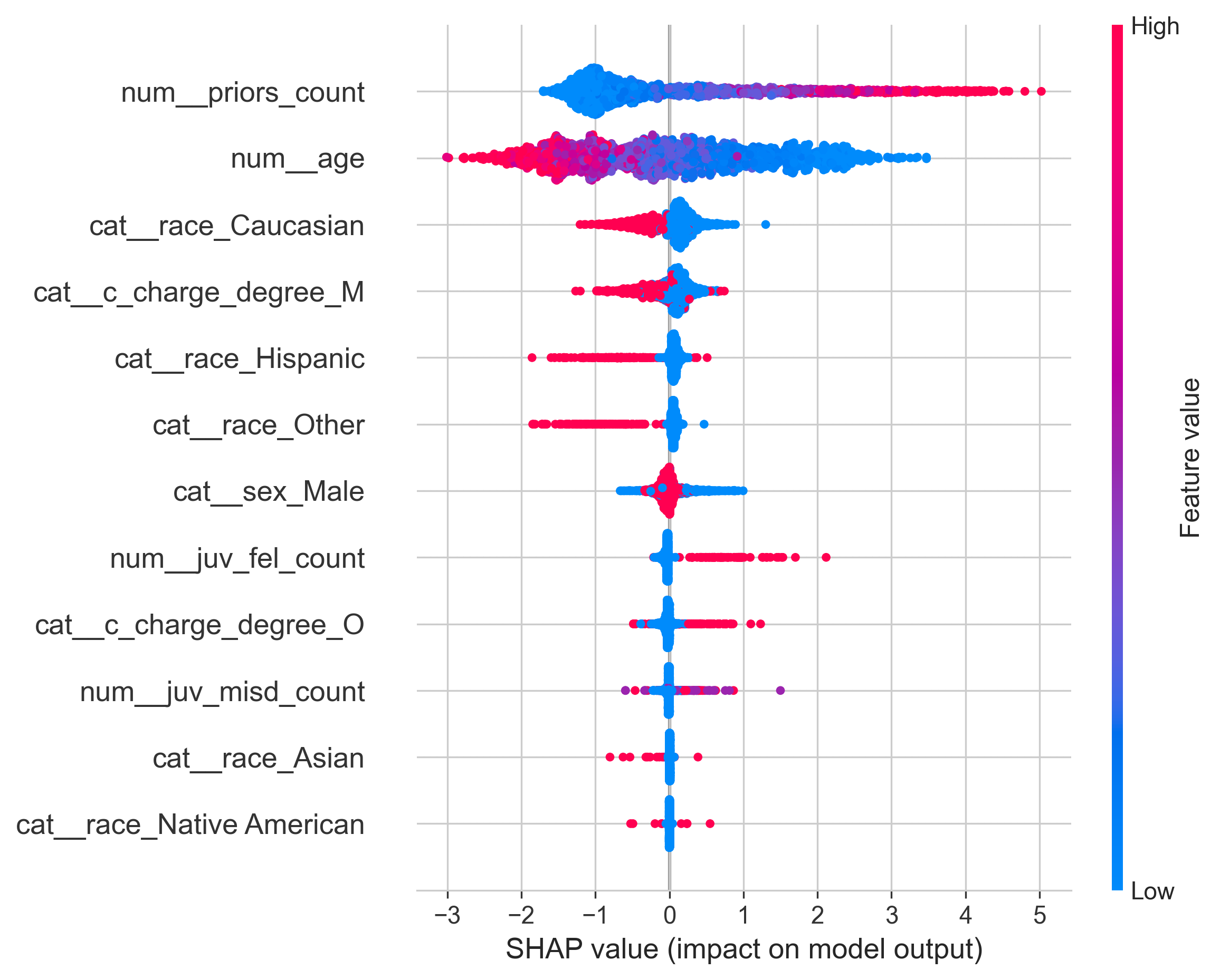
And here such results: the more person had crimes in the past, the more score he/she gets, the less age the person has, the more score become, and the less Caucasian the person, the more score he/she gets. Moreover, crimes commited in minor almost do not affect on the decision, even Felonies.
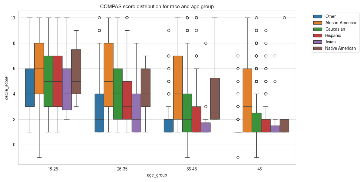
Age across races: #
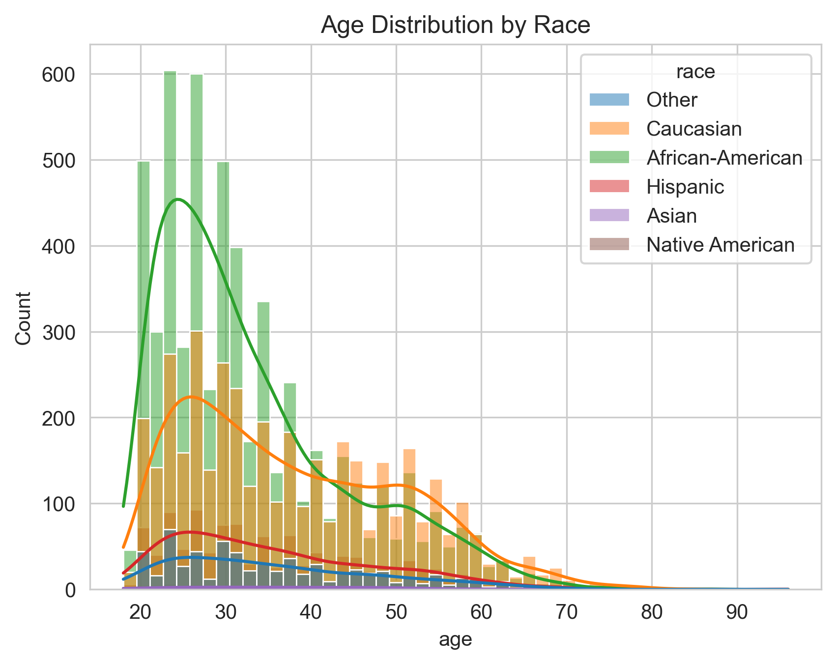
And here we see the pick of the crimes commited by African-Americans in the most discriminated groups: <25 and 26<35 y.o.
Priors across races: #
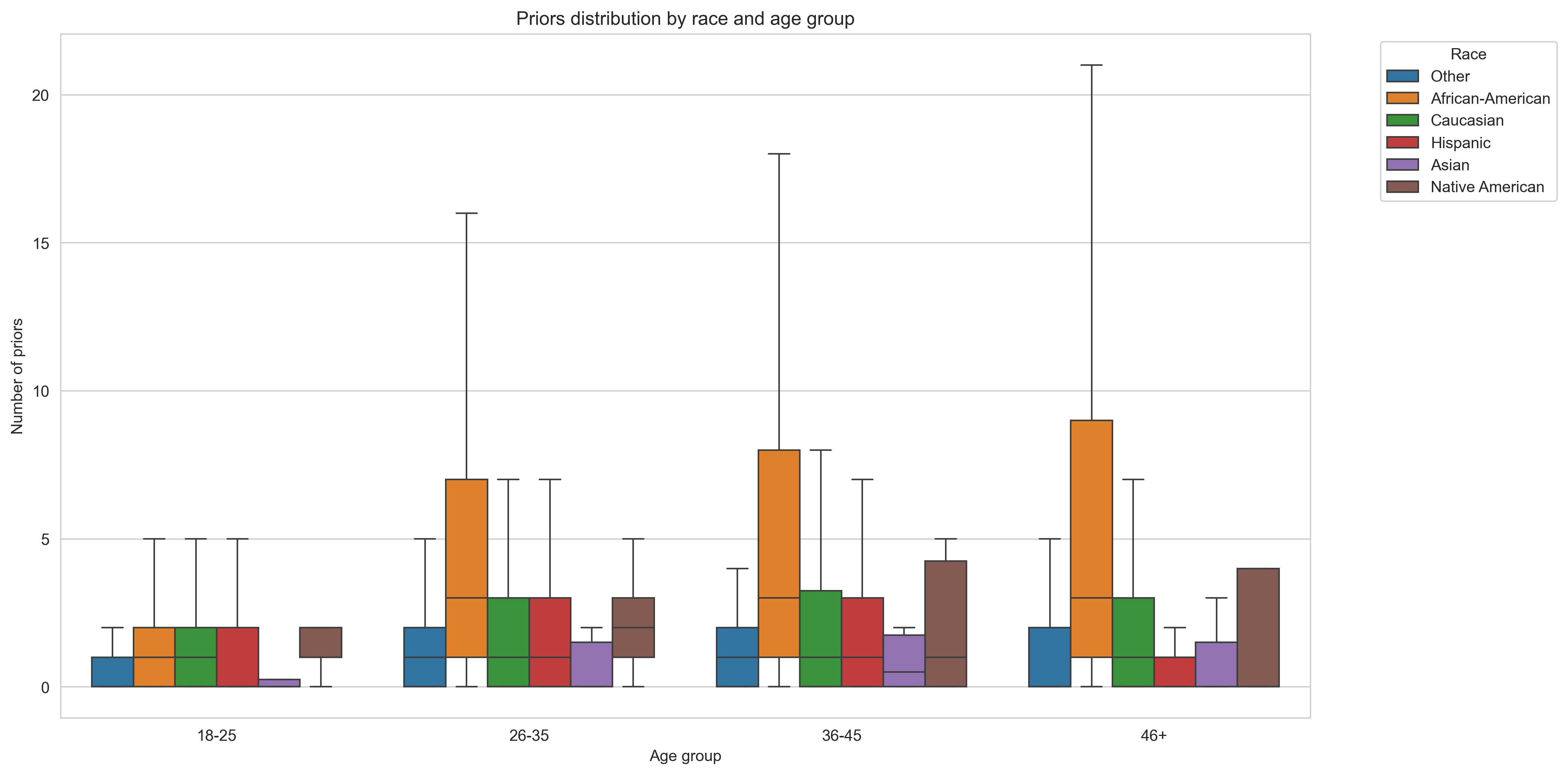
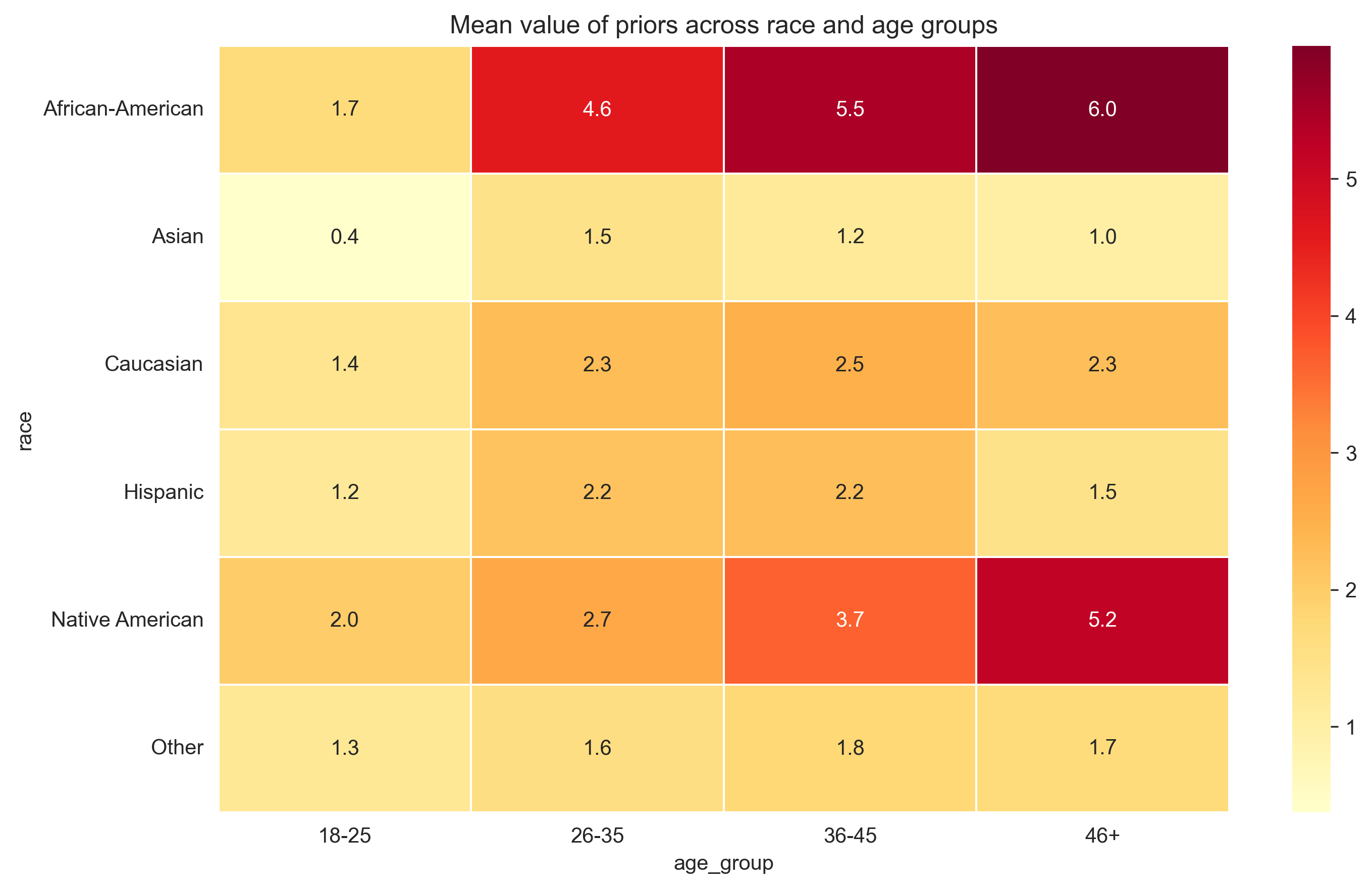
And here we see significant difference in number of previous crimes across different races.
Conclusion #
In my opinion, the model is biased because of the biased data provided in it and a prediction abstraction. The model suggests age and number of previous crimes crucial, while these two parameters are significantly differ between Caucasians and African-Americans. African-Americans have larger number of priors and they are dominant among young criminals.
But why the model suggests age as an important parameter? Because software is asked to evaluate the risk of crime in future! Not “in the next 5 years” or “in the current age group”, but just future. The model just logically assume that the younger the person - the more time he/she has to commit the crime in future. That is all.
More statistics of comparing different groups pairwise of Felony crimes provided on GitHub.
References #
[2] GitHub page