Abstract #

We introduce Integrated Hessians, the first scalable second-order attribution method for Transformer models, applying it to a RoBERTa-based sentiment classifier on the IMDb dataset. Our approach quantifies pairwise token interactions via a path-integrated Hessian, extending the axiomatic foundation of Integrated Gradients. We provide a reproducible PyTorch implementation, Dockerized environment, and visualizations (heatmaps of token–token interactions) that reveal linguistic phenomena (e.g., negation and contrast) inaccessible to first-order methods. All code is publicly available for community use and extension.

1. Introduction #

Deep NLP models such as RoBERTa achieve state-of-the-art performance but remain opaque “black boxes,” posing risks of bias, unreliability, and reduced user trust when deployed in real-world settings. Explaining model decisions is essential for transparency, fairness, and debugging. Existing gradient-based XAI methods (e.g., Integrated Gradients) provide first-order attributions of individual features but ignore pairwise interactions crucial for language understanding. We propose Integrated Hessians, extending Integrated Gradients to capture second-order effects, thereby revealing how token pairs jointly influence model outputs.

2. Background & Related Work #

2.1 Integrated Gradients #

Integrated Gradients (IG) attributes feature importance by integrating gradients along a straight-line path from a baseline \( x'\) to the input \(x\) :

IG satisfies Sensitivity and Implementation Invariance axioms but is limited to first-order effects, failing to capture interactions between features (e.g., “not” + “good”) .

2.2 SHAP #

SHAP (SHapley Additive exPlanations) unifies six existing attribution methods under a game-theoretic framework, assigning each feature a Shapley value that satisfies local accuracy, consistency, and missingness properties: \(\Large f(x) - \mathbb{E}[f(X)] = \sum_i \phi_i\) ; where \(\phi_i\) are Shapley values per feature . Kernel SHAP approximates these values for any black-box model but remains computationally expensive for large feature sets.

2.3 LIME #

LIME (Local Interpretable Model-Agnostic Explanations) fits a simple surrogate model locally around an input by perturbing features and weighting by proximity, producing an interpretable linear approximation: \(\Large \xi(x) = \underset{g \in G}{\arg\min} \; L(f, g, \pi_x) + \Omega(g)\) ; where \( L \) measures fidelity to \( f \) , \(\pi_x\) defines locality, and \( \Omega \) penalizes complexity . LIME reveals local importance but does not capture interactions.

3. Application Domain #

• Domain: Mostly(as if most commonly) sentiment analysis, but in original paper it was also used in Drug combination response prediction.

• Model: Any Transformers like BERT, RoBERTa, DistilBERT.

4. Integrated Hessians: Methodology #

4.1 Mathematical Formulation #

Integrated Gradients (First-order) #

\(\Large \text{IG}_i(x) = (x_i - x_i') \int_{\alpha=0}^{1} \frac{\partial F(x' + \alpha (x - x'))}{\partial x_i} \, d\alpha\) ;

where \(\large x \) - The input for which we’re attributing the model’s prediction,

\(\large x_i \) - The value of the i-th feature in the input,

\(\large x' \) - The baseline input (e.g., all zeros, or a neutral reference), representing the “absence” of features,

\(\large x_i \) - The value of the i-th feature in the input,

\(\large x'_i \) - The value of the i-th feature in the baseline,

\(\large \alpha \) - The interpolation constant,

\(\large \text{IG}_i(x) \) - The attribution assigned to feature i.

Integrated Hessians (Second-order) #

\(\Large \text{IH}_{i,j}(x) = (x_i - x_i') (x_j - x_j') \int_{\alpha=0}^{1} \int_{\beta=0}^{1} \frac{\partial^2 F(x' + \alpha \beta (x - x'))}{\partial x_i \, \partial x_j} \, d\beta \, d\alpha\) ;

where \(\large x_j, x'_j \) - Analogous to \(\large x_i, x'_i \) , but for feature j,

\(\large \frac{\partial^2 F(x' + \alpha \beta (x - x'))}{\partial x_i \, \partial x_j} \) - The mixed second-order partial derivative, capturing how the effect of feature i on the output changes with feature j,

\(\large \text{IH}_{i,j}(x) \) - The interaction score between features i and j.

4.2 Theoretical Advantages #

• Captures Pairwise Interactions: Explicitly quantifies how two tokens jointly influence predictions, uncovering phenomena such as negation and contrast.

• Axiomatic Foundation: Inherits completeness and sensitivity axioms from IG, extended to second-order .

• Architecture-Agnostic: Applicable to any differentiable model, including large Transformers.

5. Implementation #

• Frameworks: PyTorch, HuggingFace Transformers.

• Code Structure:

  xai_integrated_hessians/
  .
  ├── README.md
  ├── examples
  │   └── integrated_hessians_demo.ipynb      # Ipynb with demonstration
  ├── requierements.txt
  └── src
      ├── integrated_gradients.py     # contains function that calculates integrated gradients
      ├── integrated_hessians.py      # contains function that calculates hessians
      └── model_utils.py      # contains functions for plotting, proccessing and model loading
  

5.1 Calculating Integrated Gradients #

• Embeddings

input_embeddings = embeddings(input_ids)
baseline_embeddings = embeddings(baseline_ids)

These are vectors \( x \) and \( x' \)

• Interpolation

scaled_inputs = [baseline_embeddings + (float(i) / steps) * (input_embeddings - baseline_embeddings) for i in range(steps + 1)]

Generates a list of inputs from \( x' \) to \( x \) (discretization of the integral)

• Derivative

outputs = model(inputs_embeds=scaled_inputs)[0]
gradients = torch.autograd.grad(outputs.sum(), scaled_inputs)[0]

Computing for each \( \alpha \)

• Average Gradient (Riemann sum)

avg_gradients = gradients[:-1].mean(dim=0)

Approximates the integral with a Riemann sum:

• Final Attribution

attributions = (input_embeddings - baseline_embeddings) * avg_gradients

This is: \(\large\text{IG}(x) = (x - x') \cdot \text{avg\_gradients}\)

The result is a tensor of shape (1, seq_len, embed_dim).

5.2 Calculating Integrated Hessians #

• Embedding Interpolation

emb_alpha = baseline_embed + alpha * (input_embed - baseline_embed)

• First Derivative

grads = grad(score, emb_alpha, create_graph=True)[0]

• Second Derivative

grad_i = grads[0, i].unsqueeze(0)
hess = grad(grad_i, emb_alpha, grad_outputs=torch.ones_like(grad_i))[0]

• Path Integral Multiplication

delta = (input_embed - baseline_embed)[0]
ih[i] += (hess * delta).sum(dim=2).squeeze(0)

\(\Large \sum_k \frac{\partial^2 f}{\partial x_i \partial x_k} \cdot (x_k - x_k') \approx \int \frac{\partial^2 f}{\partial x_i \partial x_k} \cdot (x_k - x_k') \, d\alpha \) ;

Which is equivalent to approximation of Integrated Hessians:

• Averaging Over Steps (Riemann sum)

ih = ih * (1.0 / steps)

• Public Repo: [ GitHub link]

6. Experiments & Results #

6.1 Qualitative Insights #

• Negation: “not bad" pair of phrase “this movie was not bad” shows strong negative interaction (even though it should be positive, but for some reason pre-trained on imdb model decided that the sentiment is negative with 100% confidence)

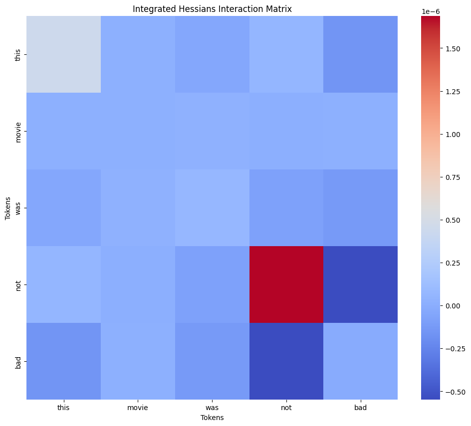
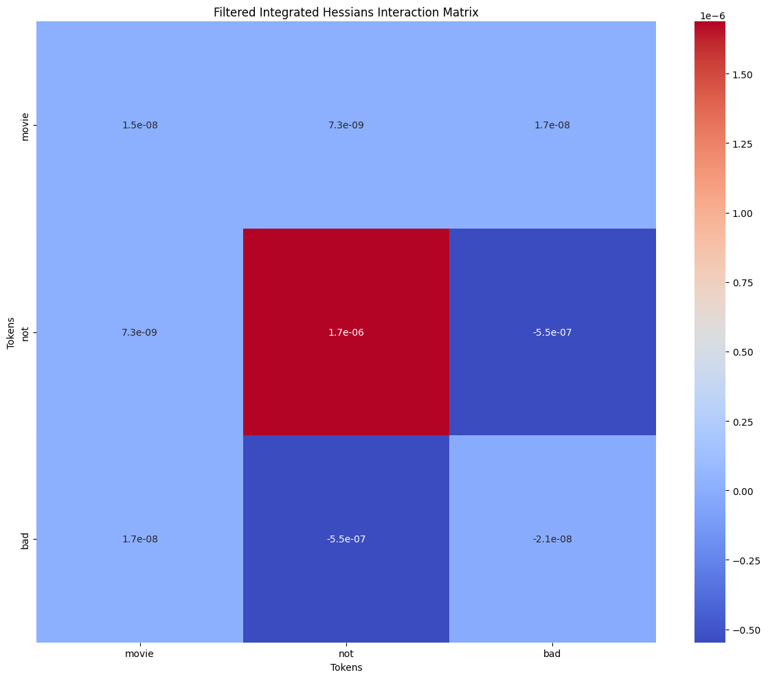
On this image you can see exact values of token interactions (some mostly meaningless tokens like punktuation is excluded), confirming that pair (not, bad) has the highest absolute value while not being on the diagonal. We don’t include the diagonal since it represents token’s intercation with itself (reminder: integrated hessians is about 2 distinct tokens interacting with each other)

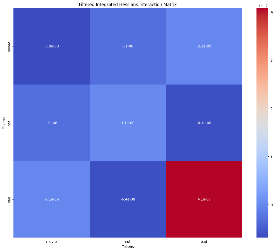
Here’s the explanation of another model’s prediction on the same phrase. This time the sentiment was predicted correctly and pair (not, bad) still had the highest value

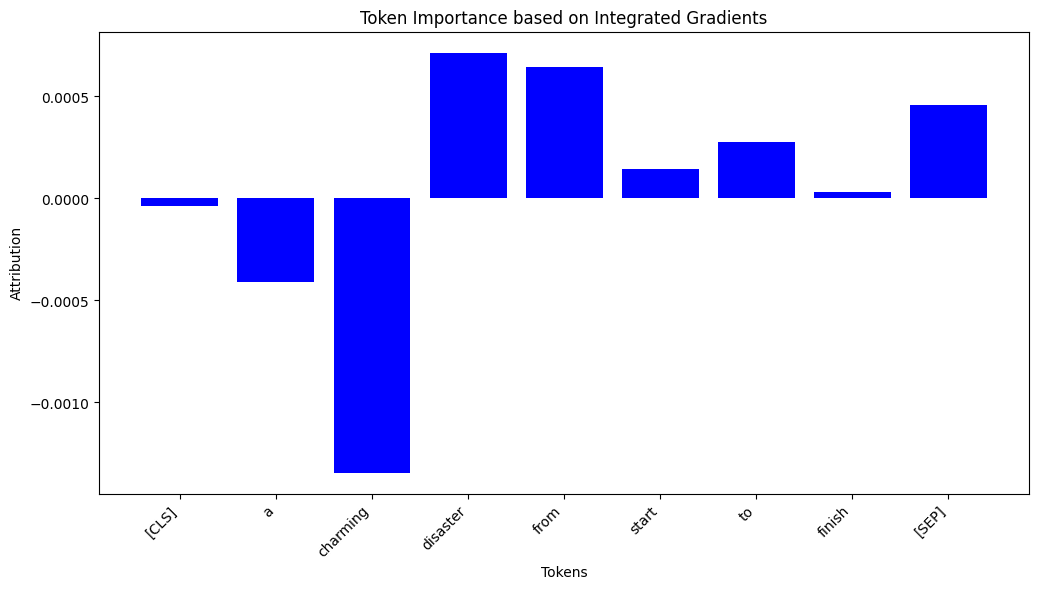
• Mixed signals: In phrase “A charming disaster from start to finish” IH highlights interaction between “charming” & “disaster”.

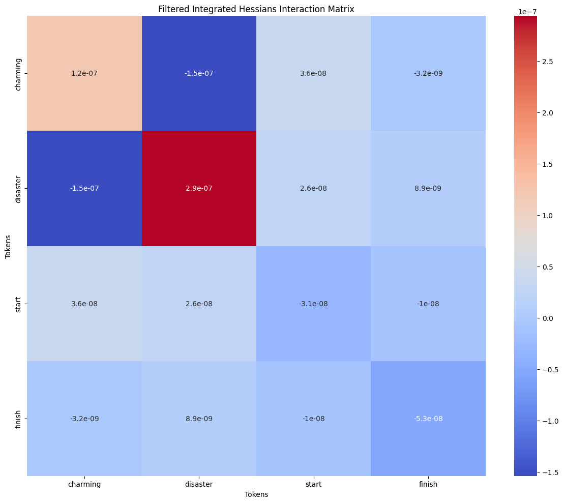
Also, Integrated Gradients show that “charming” tried to sway prediction to positive side.

7. Discussion #

• Strengths:

  • Reveals hidden linguistic structure via second-order attributions.

  • Theoretically grounded and architecture-agnostic.

• Limitations:

  • Hessian computation is computationally heavier than gradients.

  • Scalability concerns with very long sequences (quadratic in feature count).