Learnable Attention Pruning #

https://github.com/ATMI/Megatoken

Introduction #

Ever wonder how models like ChatGPT understand and generate language so well? A big part of the answer is attention — a mechanism that allows each word to adjust its meaning based on its context in a sentence.

Let’s start with a simple example:

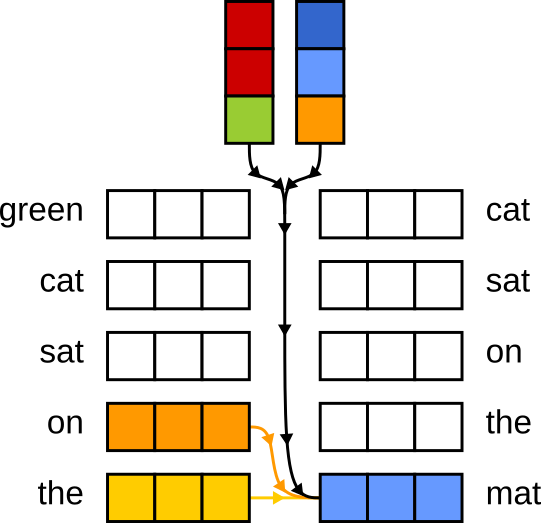
green cat sat on the mat

At first, each word is turned into a standalone vector — a numerical representation that captures its general meaning. But at this stage, the vector for cat doesn’t “know” that it’s being described as green.

That’s where attention comes in. It lets each word “look at” others in the sentence and pull in useful context. For instance, attention can update the vector for cat by blending in information from green, helping the model understand it’s not just a cat — it’s a green cat.

This context-mixing happens multiple times, each time sharpening the model’s understanding of the sentence.

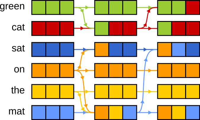
But here’s a question: once cat has absorbed info from green, do we really need to keep the green vector around? Chances are, its meaning has already been passed on. Keeping both creates redundancy — extra baggage the model has to carry.

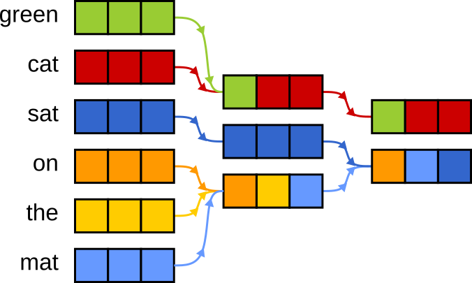
Learnable Attention Pruning is about reducing that baggage. We introduce a method that learns to drop tokens that are no longer adding value — keeping only what’s truly important.

Learnable Token Selection #

Some earlier approaches use fixed rules to decide which tokens to eliminate to produce a single output vector. Instead, we use a learnable method — one that adapts to each input and dynamically decides how many tokens to keep.

Here’s the key idea: for each token, we examine the first value in its embedding vector as a kind of importance signal. We then pass this value through a sigmoid function to get a score between 0 and 1. This score tells us how likely it is that a token should be kept in the computation.

Where:

• \(E_i[0]\) is the first element of the token’s embedding,
• \(\tau\) is a temperature parameter, which controls how sharp the selection is,
• \(\beta\) is a bias term that helps preserve more tokens early in training.

Differentiable Masking #

So how do we actually remove a token from attention?

We can’t simply delete it from the tensor. Instead, we use a mask — a special matrix that tells the model which tokens to ignore. You’ll see why this is necessary in a moment.

In transformer models, attention is computed as:

Each value in this matrix indicates how much one token attends to another. To remove a token from attention, we need to ensure its scores are effectively zeroed out. This is done using an attention mask \(M\) , which is constructed as follows:

1. Set token’s column to \(-\infty\) , so other tokens do not attend to it,
2. Set token’s row to \(-\infty\) , so it does not attend to others,
3. Set diagonal to 0, allowing the token to reference itself, which helps maintain numerical stability during softmax.

For example, to remove the first token, the attention mask would look like:

To create such masks, we define a function that depends on each token’s importance score \(\alpha_i\) :

At first glance, it might seem natural to define \(g(\alpha_i)\) with a hard threshold to achieve the same effect as removing token from tensor:

\[ g(\alpha_i) = \begin{cases} -\inf, & \alpha_i < 0.5 \\ 0, & \text{otherwise} \end{cases} \]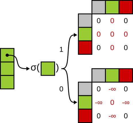

But this kind of step function isn’t differentiable — it has zero gradients everywhere, except an undefined gradient at jump point 0.5. So complete elimination isn’t suitable for training with gradient-based optimization.

To fix this, we use a smooth approximation based on the natural logarithm:

This way, we don’t remove tokens completely — we just gradually reduce their influence depending on how low their \(\alpha_i\) score is. This approach preserves differentiability and allows the model to learn which tokens matter most.

Training #

Architecture #

To train the model to compress language into a smaller set of important tokens, we use an autoencoder setup — a common architecture where an encoder learns to summarize data, and a decoder learns to reconstruct it.

But there’s a twist.

In NLP, transformer decoders need context — not just the summary from the encoder, but also the tokens they’ve already generated. This context is crucial because to generate the text, the decoder predicts just one next token at a time. Without seeing what it has generated so far, it would have no idea where it is in the sentence.

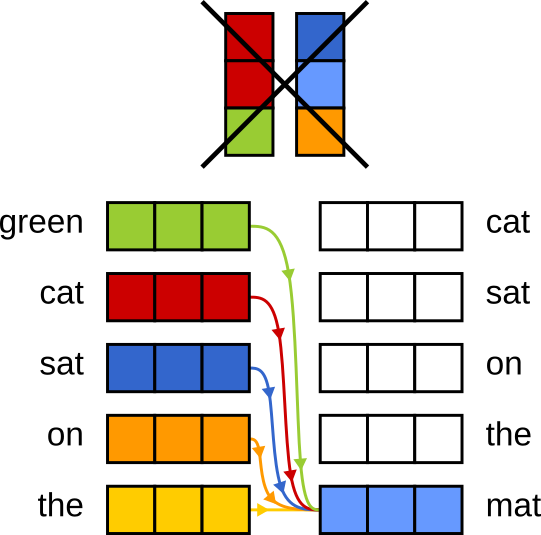
So during training, we also feed part of the original text into the decoder as context. But if we feed in too much, the decoder might ignore the encoder’s output entirely and just rely on the full original text.

To prevent this, we limit the decoder’s context to just the last \(N\) tokens — enough to help with positioning, but not enough to reconstruct the input on its own. This forces the model to actually use the encoder’s compressed memory.

Loss Function #

Our loss balances two goals: accurate reconstruction and effective compression.

Where:

1. \(\mathcal{L}_{\text{CE}}\) is the standard cross-entropy loss — it encourages the decoder to reconstruct the original text correctly,
2. \(\mathcal{L}_{\text{comp}}\) is a compression loss — it encourages the model to drop unimportant tokens,
3. \(\lambda\) controls how much we care about compression vs. accuracy.

Each token gets an importance score \(\alpha_i \in [0, 1]\) . Lower scores mean lower importance. At each step \(s\) , we track how much suppression a token accumulates over time:

Then we convert this accumulated suppression into a probability that the token still participates in the attention:

Where:

1. \(KV_{\text{dim}}\) is the dimensionality of key vector,
2. \(H\) is the number of attention heads.

The division by \(\sqrt d\) is critical: without it, modest negative values (e.g. -5) could push the exponent close to zero — suggesting a token is eliminated — even though its attention score may still be large enough to survive the masking. By scaling down the suppression term, we avoid falsely assuming a token has been removed when it hasn’t.

Now we can estimate the effective sequence length:

And compute how much it shrinks over time:

Finally, we define the compression loss:

This gives us a smooth, differentiable way to encourage shorter, more efficient representations.

Results #

We evaluated Learnable Attention Pruning using Flan-T5-small (79M parameters) on the Yelp review dataset, which contains 700K records. The model was trained for a single epoch.

Below is a plot showing how the model balances compression and accuracy during training:

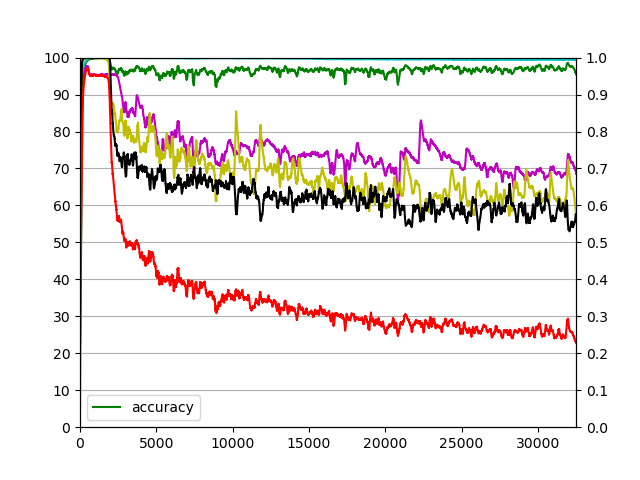
Here:

1. Green shows reconstruction accuracy — how well the decoder recreates the original text,
2. Red line tracks the overall compression ratio — how many tokens are retained vs. dropped.
3. Cyan, magenta, yellow, and black lines show compression ratios at different layers of the encoder.

To quantify performance, we measured three metrics on the test set:

These results show that Learnable Attention Pruning preserves key information while significantly reducing sequence length — achieving high fidelity reconstruction with fewer tokens.

Explainability #

Learnable Attention Pruning doesn’t just compress sequences — it preserves what matters. But how do we know the retained tokens still carry the core meaning? And how can we peek into what the model thinks is important?

To answer that, we use two tools: probing classifiers and SHAP.

Sentiment Probing #

Let’s start with a simple task: sentiment classification.

Instead of stacking a heavy model on top of our compressed sequence (which could hide the true quality of the token set), we go lightweight. We attach a small classifier — a probing head — to each token embedding and let every token “vote” on the sentiment.

Here’s how it works:

1. Each token embedding \(E_i\) is passed through a shared MLP: \[ \text{vote}_i = \text{MLP}(E_i) \]
2. We sum all the votes: \[ \text{votes} = \sum_{i=0}^{N} \text{vote}_i \]
3. And squash the result with a sigmoid: \[ P(\text{positive}) = \sigma(\text{votes}) \]

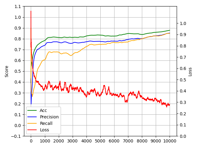
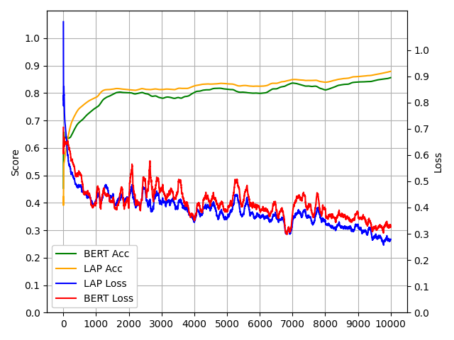
This setup lets us test whether the compressed tokens still carry enough information to capture sentiment — and they do. The performance is close to what you’d get from the standard attention-based models like BERT.

SHAP #

Okay, so the model works — but why does it make the decisions it does? SHAP gives us a lens into that.

SHAP (Shapley Additive Explanations) comes from game theory. It figures out which features are truly contributing to the output, and which are just along for the ride.

Think of each token as a player on a team. If you bench one and the model’s output sudden tanks, that token was doing important work. SHAP quantifies that impact — across all combinations of players.

Here’s the basic idea:

1. Hide different combinations of tokens from the model.
2. Watch how the model’s predictions change when each token (or group) is missing.
3. Assign a score to each token based on how much its absence affects the output — the bigger the impact, the more important it is.

Mathematically:

1. \(\phi_i\) is the SHAP value for token \(i\) ,
2. \(f(S_j)\) is the output when using subset \(S_j\) of tokens,
3. \(w_{|S_j|}\) is a weighting term for that subset size.

When we apply SHAP to Learnable Attention Pruning, we get a heatmap that shows which embeddings influence each generated token:

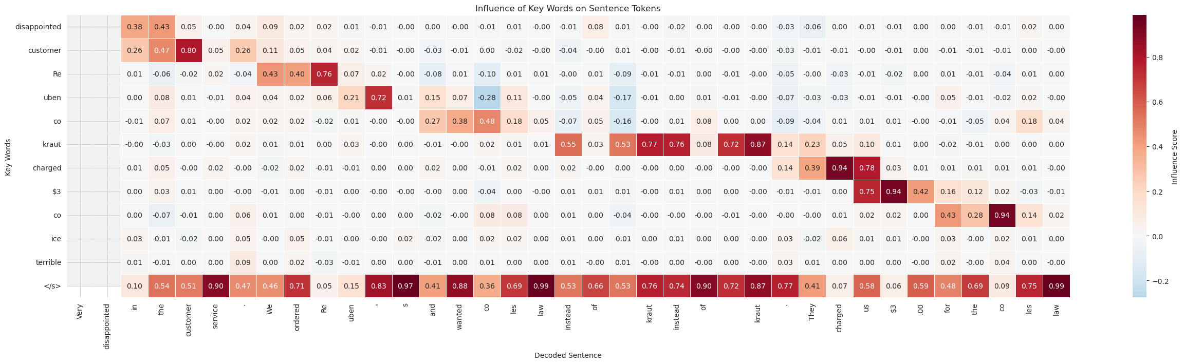
Each row is an encoder token. Each column is a generated word. Bright spots show strong influence — the pieces the model leaned on when rebuilding the output.

You’ll notice something cool: each token tends to specialize, attending to a slice of the sentence. And the final token — EOS — pulls in the big picture.

Conclusion #

Learnable Attention Pruning shows that we can reduce sequence length without losing much in terms of performance. By learning which tokens are worth keeping, the model becomes more efficient and a bit more interpretable, too.

So far, we’ve tested it on a small model and a relatively modest dataset. It would be exciting to see how this approach scales — especially with larger models, more complex data, and real-world tasks. There’s a lot of potential here, and we think this is just the start.