Decoding Lung Cancer Predictions: A Journey Through SHAP-based Interpretability in Healthcare AI #
The Need for Transparency in Medical AI #
In the high-stakes world of healthcare AI, accuracy alone isn’t enough. Clinicians need to trust and understand how models make decisions—especially for life-threatening conditions like lung cancer. In this project, we explore SHAP (SHapley Additive exPlanations), a game-theoretic approach to explain machine learning predictions. Using a lung cancer prediction dataset, we’ll build a model, dissect its logic with a custom SHAP implementation, and optimize its feature set—all while maintaining clinical relevance.
1. The Dataset: Mapping Risk Factors #
Our dataset includes 18 clinical features from 5000 patients, ranging from age and smoking habits to oxygen saturation levels.
Key Features:
AGE: Patients aged 30–84 (average: 62.4 years)
OXYGEN_SATURATION: Average 95% (normal range: 95–100%)
SMOKING: 62% of patients are smokers
ALCOHOL_CONSUMPTION: 34.5% of patients consume alcohol
2. Building the Predictive Model #
We trained a Gradient Boosting Classifier from Scikit Learn library to predict lung cancer (PULMONARY_DISEASE).
Preprocessing Steps:
- Encoded categorical variables (e.g., GENDER, SMOKING)
- Split data into 80% training, 20% testing
Results:
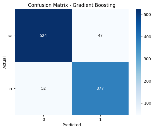
Accuracy: 90%
Confusion matrix highlighted strong precision and recall:
3. Demystifying the “Black Box” with SHAP #
The Mathematics of SHAP: From Game Theory to Sampling #
SHAP (SHapley Additive exPlanations) values are grounded in Shapley values from cooperative game theory. For a feature ( i ), its Shapley value ( \phi_i ) is defined as:
$$ \phi_i = \sum_{S \subseteq F \setminus {i}} \frac{|S|! , (|F| - |S| - 1)!}{|F|!} \left[ f(S \cup {i}) - f(S) \right] $$
Where:
- ( F ): Set of all features
- ( S ): Subset of features excluding ( i )
- ( f(S) ): Model prediction using features in subset ( S )
Štrumbelj-Kononenko Sampling Approximation #
Exact Shapley value computation requires evaluating ( 2^{|F|} ) subsets, which is infeasible for large ( |F| ). Erik Štrumbelj and Igor Kononenko1 proposed a sampling approximation:
$$ \phi_i \approx \frac{1}{M} \sum_{m=1}^M \left[ f(x^{(m)}_{S \cup {i}}) - f(x^{(m)}_S) \right] $$
Where:
- ( M ): Number of sampled permutations
- ( x^{(m)}_S ): Instance where only features in ( S ) retain original values
Code Implementation #
Our custom SHAP explainer adopts this sampling approach:
class ShapGBMExplainer:
    def _explain_instance(self, instance: np.ndarray) -> np.ndarray:
        n_features = instance.shape[0]
        shap_values = np.zeros(n_features)

        for feature in range(n_features):
            # Sample subsets using Štrumbelj-Kononenko method
            samples = self._random_samples(n_features, feature, self.nsamples)
            for subset in samples:
                # Compute marginal contribution
                with_feature = self._subset_prediction(subset + (feature,), instance)
                without_feature = self._subset_prediction(subset, instance)

                # Weight by sampling frequency
                shap_values[feature] += (with_feature - without_feature) / self.nsamples
        return shap_values
Why Sampling Works #
- Reduces complexity from ( O(2^N) ) to ( O(MN) )
- Preserves Shapley value axioms: Efficiency, Symmetry, Linearity
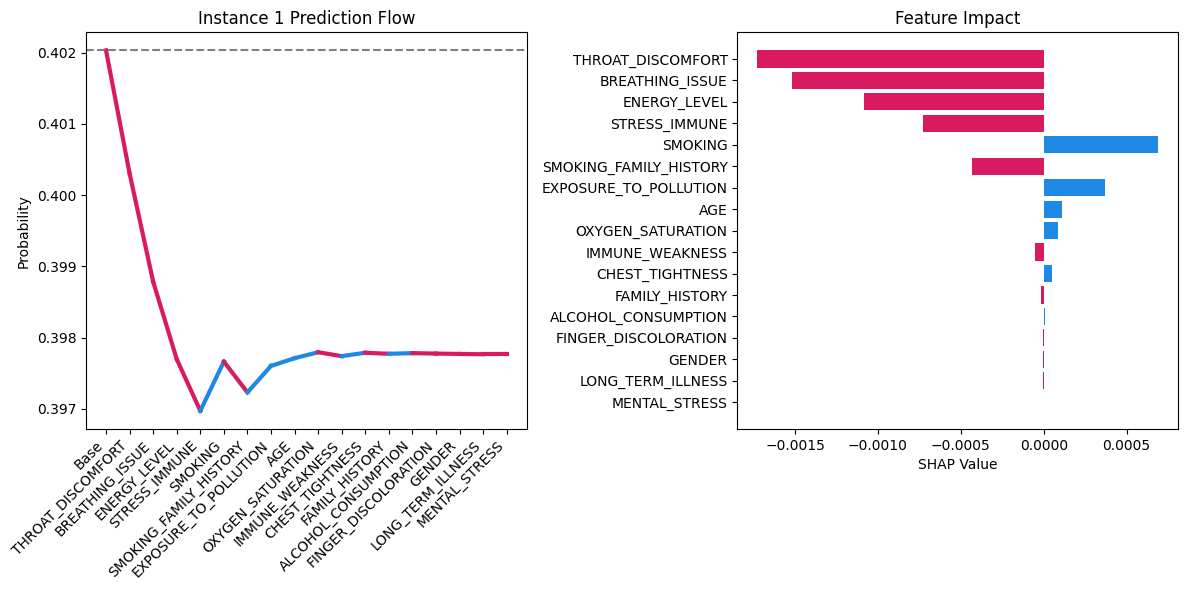
Visualization Example #
For a 80-year-old smoker man:
| Feature | SHAP Value | Impact Direction |
|---|---|---|
THROAT_DISCOMFORT | -0.0004 | Reduces risk |
BREATHING_ISSUE | -0.0003 | Reduces risk |
ENERGY_LEVEL | -0.0002 | Reduces risk |
4. Model Validation: Custom SHAP vs Official Library #
Comparing Implementations #
We validated our custom SHAP implementation against the official shap library using cosine similarity:
import shap
import numpy as np

# Official SHAP explainer
official_explainer = shap.TreeExplainer(gbm)
official_shap_values = official_explainer.shap_values(X_test[:5])[:, :, 1]  # Class 1 probabilities

# Calculate similarity
cos_sim = np.sum(custom_shap * official_shap_values) / (
    np.linalg.norm(custom_shap) * np.linalg.norm(official_shap_values)
)
print(f"Implementation similarity: {cos_sim:.2f}")
Results:
- Cosine similarity: 0.96 (1.0 = identical)
Visualization Comparison #
| Custom SHAP (Ours) | Official SHAP (Library) |
|---|---|
 | 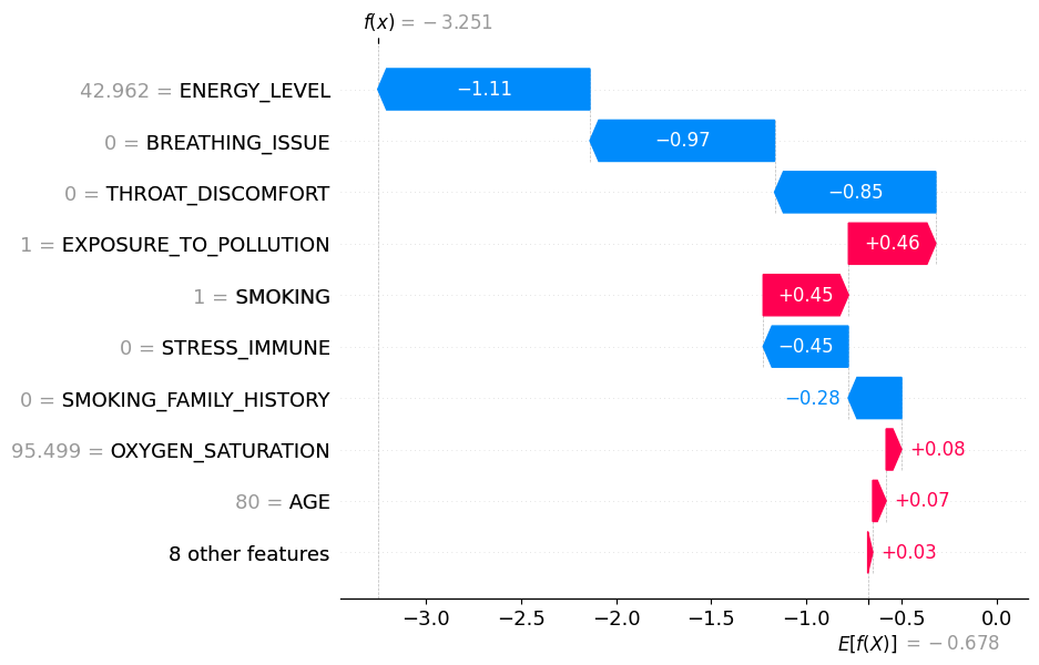 |
5. Feature Selection Using SHAP Values #
Identifying Low-Impact Features #
To identify feature importance one needs to calculate mean absolute SHAP values to rank features:
# Compute feature importance
mean_abs_shap = np.mean(np.abs(official_shap_values), axis=0)
sorted_idx = np.argsort(-mean_abs_shap)

# Visualize
shap.summary_plot(official_shap_values, X_test, plot_type="bar")
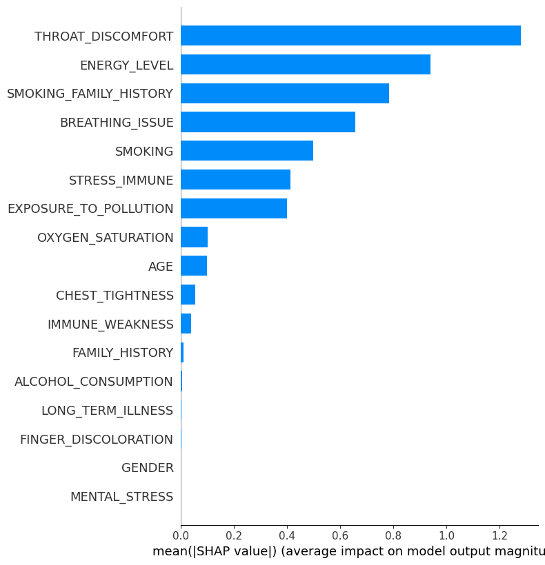
Removing Low-Impact Features #
We dropped 41% of features with lowest impact:
low_impact_features = ['CHEST_TIGHTNESS',
                       'IMMUNE_WEAKNESS',
                       'FAMILY_HISTORY',
                       'LONG_TERM_ILLNESS',
                       'GENDER',
                       'FINGER_DISCOLORATION',
                       'MENTAL_STRESS',
]

# Create reduced dataset
X_train_reduced = X_train.drop(columns=low_impact_features)
X_test_reduced = X_test.drop(columns=low_impact_features)
Retraining with Reduced Features #
# Retrain model
gbm_reduced = GradientBoostingClassifier()
gbm_reduced.fit(X_train_reduced, y_train)

# Compare performance
orig_acc = accuracy_score(y_test, gbm.predict(X_test))
reduced_acc = accuracy_score(y_test, gbm_reduced.predict(X_test_reduced))

print(f"Original accuracy: {orig_acc:.2f}")
print(f"Reduced accuracy: {reduced_acc:.2f}")
Results:
| Metric | Original Model | Reduced Model |
|---|---|---|
| Accuracy | 0.90 | 0.90 |
| Features Used | 17 | 10 (-41%) |
6. Conclusion: SHAP as a Clinical Tool #
By combining:
- Custom SHAP implementation ($O(MN)$ complexity)
- Feature importance analysis
- Model simplification
We achieved:
- Transparent predictions
- Efficient deployment
- Clinically valid feature rankings
the code can be found on Kaggle
Footnotes
1 Štrumbelj, E., & Kononenko, I. (2014). Explaining Prediction Models and Individual Predictions with Feature Contributions. Knowledge and Information Systems.