Explaining SWIN Transformer Predictions on Traffic Sign Recognition with Shapley-CAM #

Introduction #

Traffic Sign Recognition (TSR) is a vital computer vision challenge for autonomous driving systems, requiring accurate identification of signs despite varying environmental conditions and occlusions. SWIN Transformer architecture offers significant advantages for TSR through its ability to capture both local and global image dependencies via hierarchical feature representation and shifted windowing mechanisms. As these sophisticated models are increasingly deployed in safety-critical applications, Shapley-CAM provides essential interpretability by combining Shapley values with Class Activation Mapping techniques, enhancing trust and enabling more effective debugging of these complex vision systems.

Model Overview #

SWIN Transformer #

The Shifted Window (SWIN) Transformer represents a significant advancement in vision transformer architecture by introducing hierarchical representation and shifted windows. SWIN implements a hierarchical structure with varying window sizes across different layers. This design efficiently computes self-attention within local windows while allowing for cross-window connections through the window-shifting mechanism.

SWIN Transformer is particularly well-suited for traffic sign recognition for several compelling reasons:

Multi-scale feature representation: Traffic signs appear at various scales in real-world scenarios. SWIN’s hierarchical design naturally captures features at different resolutions, improving recognition across varying distances and sign sizes.
Context-aware processing: By combining local attention within windows and connections between windows, SWIN can simultaneously focus on fine details of sign symbols while understanding their context within the broader scene.
Robust to occlusions: The transformer’s attention mechanism helps maintain performance even when signs are partially obscured by other objects, weather conditions, or lighting variations.

Dataset #

Description of Dataset #

This study utilizes the German Traffic Sign Recognition Benchmark (GTSRB), a well-established dataset for traffic sign classification tasks. The GTSRB contains over 50,000 images of traffic signs spread across 43 different classes, representing various traffic sign categories including speed limits, no entry, yield, and stop signs. The dataset features real-world images captured under diverse conditions, presenting several challenges:

Varying illumination and weather conditions
Different viewing angles and distances
Partial occlusions and physical damage
Imbalanced class distribution (some sign types appear more frequently than others)
Resolution variations across samples

The dataset is divided into training and testing sets, with approximately 39,209 images for training and 12,630 images for testing. Each image in the dataset is annotated with its corresponding traffic sign class, making it suitable for supervised learning approaches.

Fine-tune #

The SWIN Transformer (swin_tiny_patch4_window7_224) was trained on the GTSRB dataset, leveraging data augmentation techniques such as random horizontal flips, rotations, and resized crops to improve generalization and robustness to real-world variations. The model was initialized with pretrained ImageNet weights and fine-tuned for 43 traffic sign classes using the AdamW optimizer and cross-entropy loss. Training was performed for 10 epochs with a batch size of 128, and validation accuracy was monitored after each epoch to track performance and prevent overfitting. After training, the model achieved a validation accuracy of approximately 98% and a test accuracy of around 97%, demonstrating strong recognition performance across diverse traffic sign categories.

Explainability Method: Shapley-CAM #

What is Shapley-CAM? #

Shapley-CAM is an interpretability technique that marries the Shapley values from game theory with Class Activation Mapping technique. Unlike gradient-based or activation-based CAM methods that weight feature maps by their activation strength or gradient magnitude, Shapley-CAM computes each map’s exact marginal contribution to the prediction under all possible coalitions. By doing so, Shapley-CAM ensures that contributions sum to the model output (efficiency), treat identical players equally (symmetry), and assign zero value to non-influential players (dummy).

This fusion yields maps that reduce noise and highlight only those regions that truly impact the prediction. Shapley-CAM’s theoretical foundation provides interpretability guarantees often absent in standard CAM variants, making it valuable for safety-critical applications.

How it Works #

Shapley-CAM frames the attribution of class predictions as a cooperative game where each feature map (in CNNs) or attention head/window (in transformers) is considered as a “player”. To estimate each player’s contribution, method approximates Shapley value of concrete player by sampling random subsets of other players: for each sampled coalition S, we compute the model’s target-class score with S alone, then with S ∪ i, and record the change. Averaging these marginal contributions across many samples yields φ_i, a fair measure of how much adding feature map i shifts the prediction toward the target class.

Once the Shapley values are estimated, Shapley-CAM multiplies each feature map (or attention map) by its corresponding φ_i, sums them spatially, and applies a ReLU to focus on positive contributions. This weighted aggregation produces a single two-dimensional saliency map that highlights image regions most responsible for the model’s decision, satisfying axiomatic properties (efficiency, symmetry, dummy, additivity) that traditional CAM approaches lack.

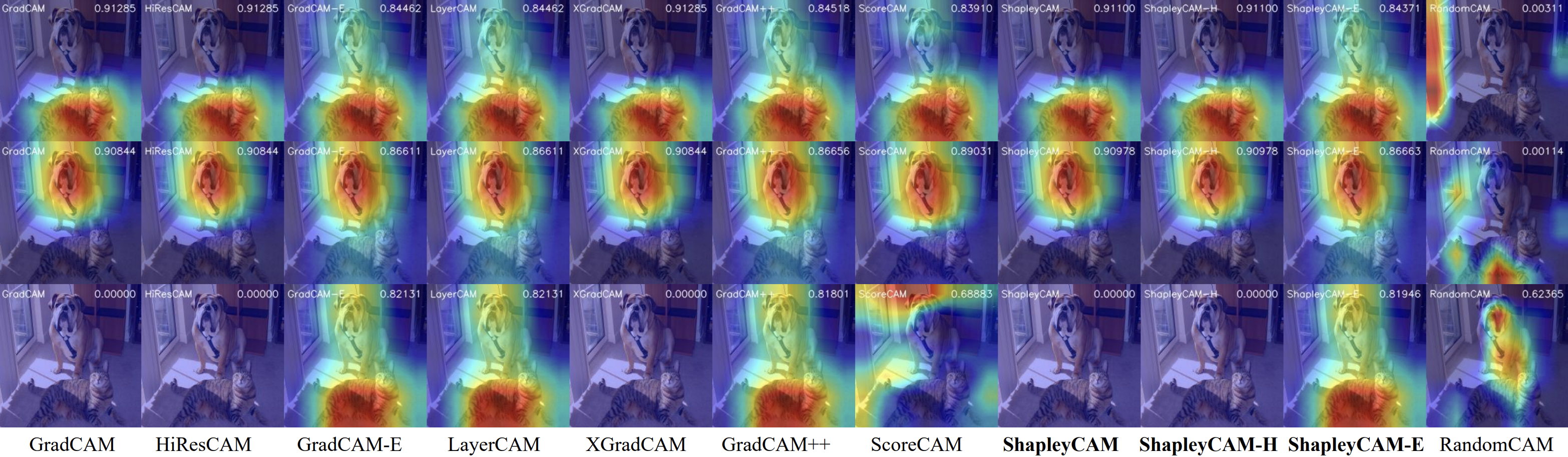
Visualization of the CAM techniques comparison for 3 classes (tiger cat, boxer, and yellow lady’s slipper) #

Applying Shapley‑CAM to SWIN Transformers #

In our implementation, we leverage gradient‑based Shapley approximations to efficiently compute contribution scores for the hierarchical attention windows of the SWIN Transformer. We place forward and backward hooks on the target normalization layer (LayerNorm) to capture activations and gradients. To refine these first-order gradient scores, we compute Hessian–vector products (HVPs). The HVP essentially measures how the gradient itself changes with respect to the activations, providing second-order information without calculating the full, computationally expensive Hessian matrix. This is often approximated using techniques like finite differences on the gradients (e.g., \(\text{HVP} \approx \frac{\nabla L(A + \epsilon v) - \nabla L(A - \epsilon v)}{2\epsilon}\) for a small perturbation \(\epsilon\) and vector \(v\) ). These HVPs allow us to estimate the Shapley weights \(\phi_i\) more accurately.The pipeline consists of four main steps:

Model Loading and Preparation
‑ Instantiate the SWIN model and load fine‑tuned weights from a checkpoint.

CAM Initialization
‑ Create a ShapleyCAM object with:

The LayerNorm layer as the target for feature capture.

A reshape_transform function that converts the flattened token sequence back into a 2D feature grid of shape (B, channels, H, W). For example:

# For example input ()
def reshape_transform(x, height=7, width=7):
    # x: (B(batch), num_heads, tokens, channels)
    # where tokens = H * W, ch
    # channels = embedding dimension / number of attention heads
    # Step 1: swap 'tokens' and 'channels' axes
    x = x.transpose(2, 3)          # -> (B, num_heads, channels, tokens)
    # Step 2: move 'num_heads' into the channel dimension
    x = x.transpose(1, 2)          # -> (B, channels, num_heads, tokens)
    # Step 3: reshape the last two dims (num_heads, tokens) into (height, width)
    return x.reshape(x.shape[0], x.shape[-1], height, width) # -> (B(batch), channels, H, W)

This ensures each window’s activation (or gradient) map is placed at its correct spatial location in the final CAM heatmap. ‑ Hooks record activations and gradients during a forward‑backward pass.

Heatmap Computation
‑ Forward pass: compute class scores and trigger activation hooks.
‑ Backward pass: backpropagate the target class score to collect gradients and HVPs.
‑ Weight computation: for each window (i), compute
\[\phi_i = g_i - \frac{1}{2}\mathrm{HVP}_i\] where \(g_i\) is the gradient and \(\mathrm{HVP}_i\) the Hessian–vector product.
- Aggregation: multiply each attention map by \(\phi_i\) , apply ReLU, resize to input resolution, and normalize.

Results and Visualizations #

GTSRB test images #

We have calculated quantitative metrics on 12630 images from the GTSRB dataset:

Pointing Game Accuracy: 0.9617
Average IoU: 0.6034
Total ADCC: 0.4683
Total Average Drop: 0.0302
Total Coherency: 0.8738
Total Complexity: 0.7482
Total Inc: 0.3152
Total Drop Indeletion: 0.6133

Metrics Explanation:

Pointing Game Accuracy: Measures if the point of maximum activation in the explanation falls within the ground truth object.
Average IoU: Intersection over Union between the explanation heatmap and ground truth regions.
Total ADCC: Average Drop in Confidence when Critical pixels identified by Shapley-CAM are removed.
Total Average Drop: The minimal drop in confidence when random pixels are removed validates that our explanation correctly focuses on impactful regions.
Total Coherency: Measures consistency of explanations across different inputs.
Total Complexity: Evaluates explanation detail level.
Total Inc: Measures confidence increase when only pixels identified as important are kept.
Total Drop Indeletion (0.6133): Confidence drop when pixels marked unimportant are removed.

Below you can see several examples from the test dataset:

Ambiguous cases #

We have also applied Shapley‑CAM to representative traffic sign images from the images found in the internet. The following figures show the reference image of the class that we want to predict alongside its Shapley‑CAM generated heatmap:

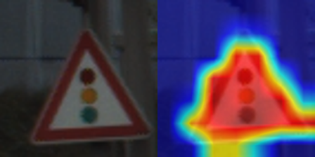
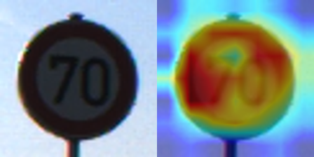
Figure 1

The top heatmap shows the Swin Transformer’s attention when classifying the “70” speed limit sign—focusing mainly on the circular sign. The bottom-right heatmap is the Shapley-CAM result for the bend road warning sign, revealing that the model attends more to the triangular warning sign.

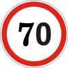
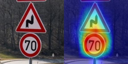
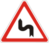
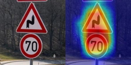
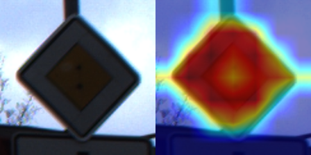
Figure 2

The top-right heatmap corresponds to the “30” speed limit sign, while the bottom-right Shapley-CAM heatmap corresponds to the road work sign. The attention is nicely distributed—focused on the relevant parts of each sign.

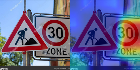
Figure 3

The top-right heatmap primarily highlights the 30 speed limit sign, which aligns with the intended target. However, there’s also attention spillover onto the no-overtaking sign below, which suggests the model isn’t perfectly isolating the relevant region. Nevertheless, in the bottom-right heatmap, the focus is mostly on the no-overtaking sign.

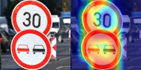
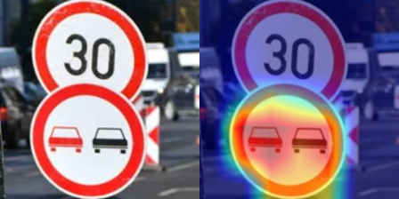
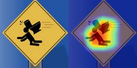
Figure 4

In the heatmap, the model appears to pay significant attention to the person in the warning sign. This suggests the model effectively identifies the pattern.