Explaining Neural Networks with SmoothGrad #

This project implements and explores gradient-based explanation methods for neural networks, with a particular focus on SmoothGrad and how it improves upon vanilla gradient and integrated gradient methods.

Introduction #

Neural networks have achieved remarkable success in various domains, but their black-box nature often makes it difficult to understand how they make decisions. Saliency maps are one approach to address this challenge by highlighting regions in the input that have the most significant influence on the model’s predictions.

This repository provides implementations of three key saliency map generation techniques:

Vanilla Gradients
Integrated Gradients
SmoothGrad (which can be applied to any gradient-based method)

Vanilla Gradients #

The vanilla gradient method is the simplest approach to generating saliency maps. It works by:

Forward propagating an input through the neural network
Calculating the gradient of the output with respect to the input
Taking the absolute value of these gradients
Averaging across the color channels (for images)

Mathematically, for an input x and a model f, the vanilla gradient saliency map is:

\[$$S(x) = \left|\frac{\partial f(x)}{\partial x}\right|$$\]

Limitations: While simple to compute, vanilla gradients often produce noisy and scattered saliency maps that can be difficult to interpret. They tend to highlight edges rather than the complete objects of interest.

Integrated Gradients #

Integrated Gradients (IG) addresses some of the limitations of vanilla gradients by considering the path integral from a baseline input to the actual input. It computes:

\[$$IG(x) = (x - x_0) \times \int_{\alpha=0}^{1} \frac{\partial f(x_0 + \alpha(x - x_0))}{\partial x} d\alpha$$\]

Where:

$x$ is the input
$x_0$ is a baseline input (often zero or random noise)
$\alpha$ is a scaling factor along the path from baseline to input

In practice, the integral is approximated using a Riemann sum:

\[$$IG(x) \approx (x - x_0) \times \frac{1}{m} \times \sum_{i=1}^{m} \frac{\partial f(x_0 + \frac{i}{m}(x - x_0))}{\partial x}$$\]

Advantages:

Satisfies the completeness axiom - the attributions add up to the difference between the output at the input and baseline
More theoretically sound than vanilla gradients
Often produces more cohesive attribution maps

Limitations:

Computationally more expensive than vanilla gradients
Still can produce noisy results
Sensitive to the choice of baseline

SmoothGrad: A Monte Carlo Approach #

SmoothGrad is a technique that can be applied to any gradient-based attribution method to reduce noise and create more visually coherent saliency maps.

Principles of SmoothGrad #

The key insight behind SmoothGrad is that gradient-based explanations are often noisy due to the high non-linearity of neural networks. Small perturbations in the input can lead to large changes in the gradient, creating scattered and hard-to-interpret saliency maps.

SmoothGrad addresses this by:

Adding random Gaussian noise to the input sample multiple times
Computing saliency maps for each noisy sample
Averaging these maps to produce a smoother result

Mathematically:

\[$$SmoothGrad(x) = \frac{1}{n} \sum_{i=1}^{n} S(x + \mathcal{N}(0, \sigma^2))$$\]

Where:

$S$ is any saliency map generation function (like vanilla gradients or integrated gradients)
$n$ is the number of samples
$\mathcal{N}(0, \sigma^2)$ is Gaussian noise with standard deviation $\sigma$

Connection to Monte Carlo Methods #

SmoothGrad is fundamentally a Monte Carlo method because:

Sampling Approach: It uses random sampling to estimate an expectation. In this case, it samples from the distribution of inputs perturbed by Gaussian noise.
Law of Large Numbers: As the number of samples increases, the average of the saliency maps converges to the expected value of the saliency map under the noise distribution.
Variance Reduction: Like other Monte Carlo methods, increasing the number of samples reduces the variance in the estimated saliency map, leading to smoother and more stable results.

This Monte Carlo approach makes SmoothGrad particularly effective at reducing the visual noise in gradient-based explanations while preserving the important features that truly influence the model’s predictions.

Implementation Details #

project link

Our implementation of SmoothGrad can be applied to any gradient-based method by wrapping the base method:

# Apply SmoothGrad to vanilla gradients
smooth_vanilla = SmoothGrad(
    base_grad_class=BaseGrad(model),
    std=0.15,        # Standard deviation of the noise
    n_samples=50     # Number of samples to average
)

# Apply SmoothGrad to integrated gradients
smooth_integrated = SmoothGrad(
    base_grad_class=IntegratedGradients(model, n_steps=5),
    std=0.15,
    n_samples=50
)

Key parameters:

base_grad_class: The base gradient method to enhance
std: Standard deviation of the Gaussian noise (controls how much variation is introduced)
n_samples: Number of noisy samples to generate (higher values give smoother results but increase computation time)
perturb_batch_size: Batch size for processing noise samples (for computational efficiency)

Comparison of Methods #

When applied to image classification tasks, SmoothGrad consistently produces more interpretable saliency maps compared to the vanilla methods:

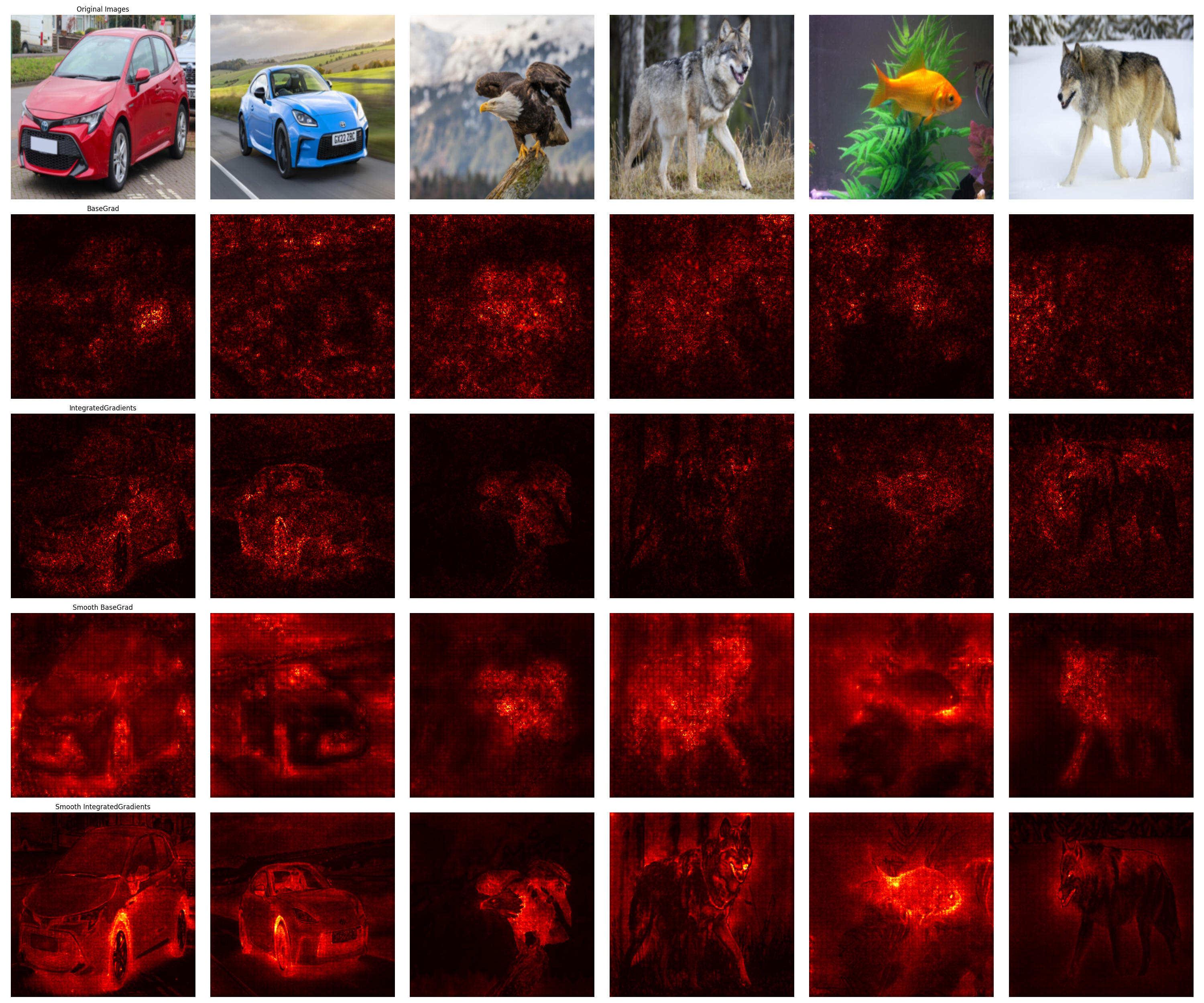Comparison of saliency methods Comparison of different saliency map methods: Vanilla Gradients, Integrated Gradients, and their respective SmoothGrad versions.

Vanilla Gradients vs. SmoothGrad #

Vanilla Gradients: Often highlight edges and produce scattered, noisy maps that are difficult to interpret
Smooth Vanilla Gradients: Produce more cohesive maps that highlight the complete objects or regions of interest

Integrated Gradients vs. Smooth Integrated Gradients #

Integrated Gradients: Provide better attributions than vanilla gradients but can still be noisy
Smooth Integrated Gradients: Combine the theoretical advantages of integrated gradients with the noise reduction of SmoothGrad

The visual difference is often striking - while vanilla methods may highlight scattered pixels across an image, SmoothGrad methods tend to produce more focused, cohesive regions that better align with human intuition about what parts of the image are important for classification.

Conclusion #

SmoothGrad represents a significant improvement in the interpretability of neural networks through its application of Monte Carlo principles to gradient-based explanations. By averaging saliency maps over multiple noisy samples, it produces smoother, more visually coherent explanations that better identify the regions of input that truly influence a model’s predictions.

This project demonstrates how SmoothGrad can be combined with different base methods (vanilla and integrated gradients) to enhance their effectiveness, providing researchers and practitioners with more reliable tools for understanding and explaining neural network decisions.

Usage #

To compare different saliency methods on your own images:

from src.grads import BaseGrad, IntegratedGradients, SmoothGrad
from src.utils import compare_saliency_methods, create_dataset

# Load your model and dataset
model = ...  # Your neural network model
dataset = create_dataset("path/to/images_folder", device="cuda")

# Create gradient methods
base_methods = [
    BaseGrad(model),
    IntegratedGradients(model, n_steps=5)
]

# Create smooth versions
smooth_methods = [
    SmoothGrad(BaseGrad(model), std=0.15, n_samples=50),
    SmoothGrad(IntegratedGradients(model, n_steps=5), std=0.15, n_samples=50)
]

# Compare methods
compare_saliency_methods(dataset, base_methods, smooth_methods)

This will generate a grid of visualizations showing the original images along with their corresponding saliency maps for each method, similar to the comparison image shown above.