Explaining Reinforcement Learning with Shapley Values | Tutorial #
Introduction #
Explainability and interpretability of AI models is a hot topic in the research community in recent times. With the growth of new technologies and methods in the neural networks field, the endeavour to understand the “black box” models is rising in popularity.
In this tutorial, you will learn 2 methods for explaining the reinforcement learning models:
- Applying Shapley values to policies
- Using SVERL-P method
Before we start, this tutorial is based on the paper “Explaining Reinforcement Learning with Shapley Values” by Beechey et. al. [1], where the researchers present 2 approaches on how to explain reinforcement learning models with Shapley values.
Also, we assume that you are familiar with machine learning, reinforcement learning, but not familiar with explainable artificial intelligence.
A quick reminder: reinforcement learning is a type of unsupervised learning technique, in which you train the agent in the environment, which can vary from a hide-and-seek game to a traffic simulation.
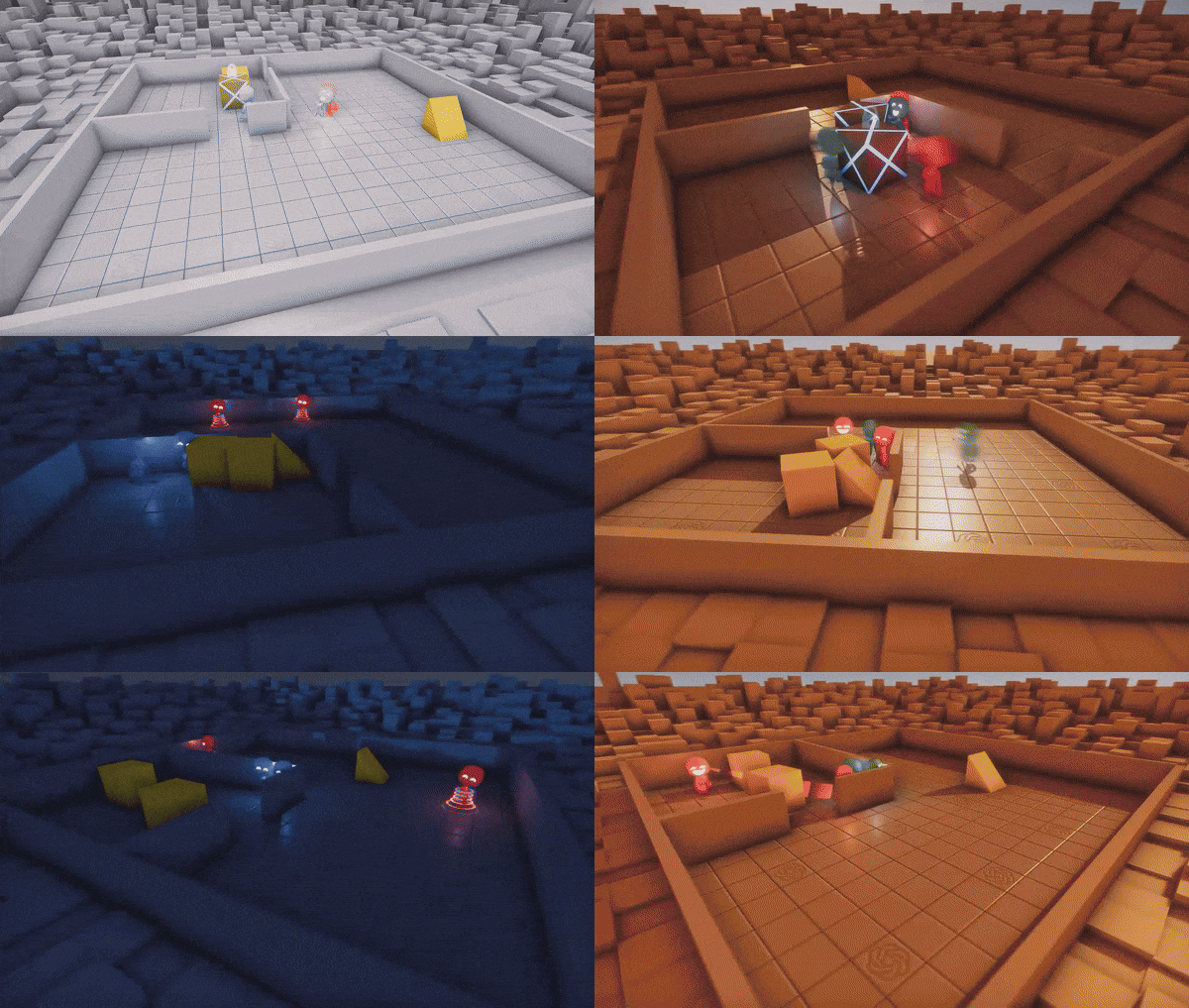
OpenAI reinforcement learning research paper visualisation [2].
For the implementation, we will be using a ⚡blazingly fast⚡ and statically-typed programming language called 🦀 Rust 🦀. We will provide a few code snippets, but our main goal is to provide you with the idea on implementation, so you can try to implement these methods in your favourite programming language.
Explainable Artificial Intelligence #
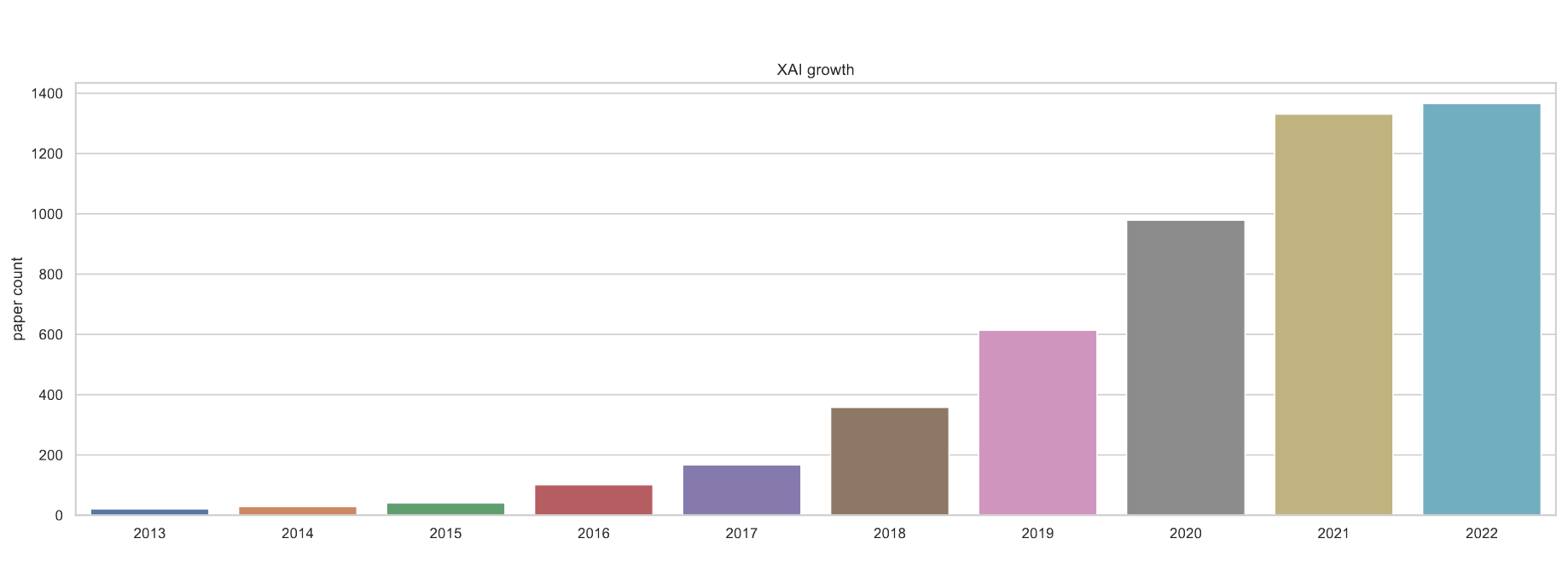
Yearly growth trends. Papers before 2013 were omitted for readability [3].
Explainable Artificial Intelligence (XAI) is a field of study that seeks to make AI systems more understandable and interpretable to humans [4].
Interpretability is the ability of a human to understand the reasoning behind a decision made by an AI system [4].
Fair AI: AI systems can perpetuate and amplify existing societal biases if they are not carefully designed. Fair AI techniques can help to ensure that AI systems make decisions that are fair and unbiased for all people [4].
There are many techniques, methods, and algorithms invented in recent years to explain AI and design it to be fair. These techniques involve: LIME (Locally Interpretable Model-Agnostic Explanations), SHAP (Shapley Additive exPlanations), DeepDream, SVERL-P, and many more.
Shapley values #

Imagine you and your friend are making a group project in a university course. At the end of the course, you get B and your friend gets A. You think this is unfair, but how to prove it? Well, to fairly assess your performance, you can calculate your contribution to the group project, i.e. to a coalition of two players using Shapley values. For example, if your friend would do the project alone, they would complete 45% of the project. However, together you complete 100% of the project.
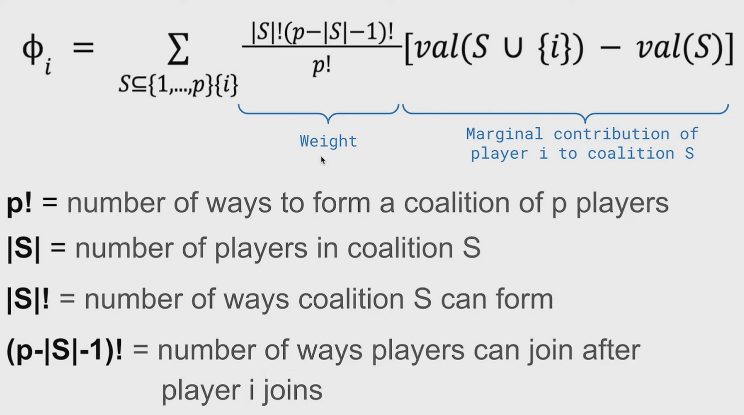
Shapley value formula [5].
Shapley values are a concept from cooperative game theory that provides a way to fairly distribute the marginal gains among players in a coalition, ensuring that each player gets as much or more than they would have if they acted independently.
In the above formula, your friend’s val(S) = 75, and the value of both of you is val(S union {i}) = 100. Now, your marginal contribution to the coalition of two players (you and your friend) is 100 - 45 = 55. Now, you cannot say that your whole contribution is 55, you need to calculate the average of this number to fairly assess your performance. That is when weight comes into play. You can think of it as a way to normalise marginal contribution over all possible coalitions, even when it is an empty coalition, i.e. noone does the project.
After all the calculations are done, you get a fair assessment of your performance, and prove to your teaching instructor that you deserve a better grade.
One more thing about Shapley values is that they satisfy the following 4 properties [6]:
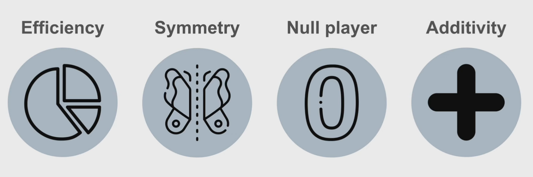
4 properties of Shapley values [5].
- Efficiency - the sum of the Shapley values of all agents equals the value of the grand coalition, so that all the gain is distributed among the agents.
- Symmetry - two players are considered interchangeable if they make the same contribution to all coalitions.
- Null player - if the player makes 0 contribution to all coalitions, then they have zero shapley value.
- Linearity (Additivity) - shapley value of coalition is equal to shapley values of individuals in this coalition.
Environment #
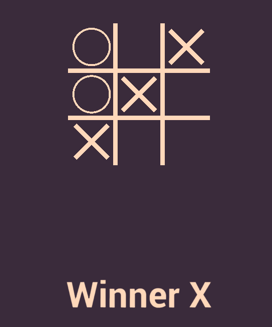
For this project, we have coded the Tic-Tac-Toe game in the Rust programming language using Geng game engine [7].
In the centre of the screen there is a grid of cells, where each cell contains either: nothing, cross, or circle. Players make moves in-turns, and one of them wins if they either make a consequent horizontal, vertical, or diagonal line of the same shape, corresponding to them (circle or cross).
Exact implementation of this environment is out of scope for this tutorial. However, you can find the full source code on our GitHub [8].
In this simple environment we will introduce 2 models/policies and try to interpret their actions. For that reason, we first need to describe the environment in terms of Markov Decision Process:
- State is the grid, consisting of 9 cells.
- Action is an input from the user to place a shape. In our case, we have 9 actions, one for each cell. Environment handles the turns automatically, so that is why you do not need to worry about which shape to put.
- Reward is either 0 or 1 (player either wins a game or looses)
- Policies: random and minimax.
- Random policy outputs a random legal move, i.e. it cannot place a shape on the occupied cell or make turns when the game is finished.
- Minimax calculates all possible game outcomes for both players, and compares them. As output it produces the action, which leads to a maximum available value.
pub enum Tile {
    Empty,
    X,
    O,
}

pub struct Grid<T = Tile> {
    pub cells: [[T; 3]; 3],
}

pub type Policy = Box<dyn FnMut(&Grid) -> Grid<f64>>; // policies return the probabilty distribution over possible action
pub type Action = vec2<Coord>;
Shapley values applied to policy #
Before applying the method, we need to define terms and try to understand them.
- Policy takes a state and returns the probability distribution over possible actions.
- Observation is the state with some of the features (cells) hidden.
The first method to interpret the reinforcement learning model is to apply shapley values directly to the policy,
The value function used to evaluate a policy, as defined in the paper, is the expected probability of each action over the distribution of possible states (given current partial observation).
\(v^\pi(C) = \pi_c(a|s) = \sum_{s' \in S} p^\pi(s'|s_C) \pi(a|s') \)Where C is the observation (with the features from the coalition), \(p^\pi(s’|s_C)\) is the probability of seeing state \(s’\) given the observation \(s_C\) .
So, to calculate the Shapley value for each feature for every action, we first need to get all partial observations:
impl Grid {
    pub fn all_subsets(&self) -> Vec<Observation> {
        let positions: Vec<_> = self.positions().collect();
        powerset(&positions)
            .into_iter()
            .skip(1) // Skip the set itself
            .map(|positions| Observation {
                positions,
                grid: self.clone(),
            })
            .collect()
    }
}
Then, for every observation we calculate the value function for it and for the observation without the feature we’re calculating for:
let observations = grid.all_subsets();
let n = grid.positions().count(); // number of all features
observations
    .iter()
    .cloned()
    .map(|observation| {
        let base_value = value(feature, &observation);
        let s = observation.positions.len();
        let scale = factorial(s) as f64 * factorial(n - s - 1) as f64 / factorial(n) as f64;

        let featureless = observation.subtract(feature);

        let mut value = base_value - value(feature, &featureless);
        value *= scale;
        value
    })
    .fold(Grid::zero(), Grid::add)
The value function itself is the expected value for every action, and is easy to implement. But we also need to calculate possible states given the observation. We can do that by iterating over all hidden cells in the grid and checking all 3 possible states for that cell.
impl Observation {
    pub fn value(&self, policy: &mut Policy) -> Grid<f64> {
        let states = self.possible_states();
        let scale = (states.len() as f64).recip();

        let mut result = states
            .into_iter()
            .map(|state| policy(&state))
            .fold(Grid::zero(), Grid::add);
        result *= scale;
        result
    }

    pub fn possible_states(&self) -> Vec<Grid> {
        let hidden: Vec<_> = self
            .grid
            .positions()
            .filter(|pos| !self.positions.contains(pos))
            .collect();

        (0..3usize.pow(hidden.len() as u32))
            .map(|i| {
                let mut grid = self.grid.clone();
                for (pos, cell) in hidden.iter().enumerate().map(|(t, &pos)| {
                    let cell = match (i / 3_usize.pow(t as u32)) % 3 {
                        0 => Tile::Empty,
                        1 => Tile::X,
                        2 => Tile::O,
                        _ => unreachable!(),
                    };
                    (pos, cell)
                }) {
                    grid.set(pos, cell);
                }
                grid
            })
            .collect()
    }
}
SVERL-P #
Instead of applying shapley values directly to policy, we can use a better approach, which is called Shapley Values for Explaining Reinforcement Learning Performance or in short SVERL-P.
SVERL-P is divided into 2 methods: local and global ones.
Local SVERL-P is essentially a prediction of the reward given uncertainty of the current observation.
\(v^{local}(C) = E_{\hat\pi}[\sum_{t=0}^\infty \gamma^t r_{t+1} | s_0=s]\)Where
\(\hat\pi(a_t|s_t) = \begin{cases} \pi_C(a_t|s_t)\ if\ s_t=s, \\ \pi(a_t|s_t)\ otherwise \end{cases}\)\(r\) is the reward (winner gets the reward of 1), \(\gamma\) is the discounting factor.
Global extends the uncertainty to all future states, rather than just the starting one.
\(v^{global}(C) = E_{\pi_C}[\sum_{t=0}^{\infty} \gamma^t r_{t+1} | s_0=s]\) \(Ф_i(v^{global}) = E_{p^\pi(s)}[\phi_i(v^{global}, s)]\)Where \(\phi_i\) is the Shapley value.
The difference with the previous (regular Shapley) value function is the future prediction. So, after calculating the initial \(\pi_C\)
the same way (Observation::value), we recursively go through all the states in the future and calculate the expected reward, according to the policy action distribution.
impl Grid {
    fn predict(&self, gamma: f64, policy: &mut Policy) -> f64 {
        let Some(player) = self.current_player() else {
            return 0.0; // The game has ended
        };

        let mut result = 0.0; // Expected reward
        let weights = policy(self); // action probability distribution
        for pos in self.empty_positions() {
            let prob = weights.get(pos).unwrap();

            let mut grid = self.clone();
            grid.set(pos, player.into());

            let immediate_reward = grid.reward(player);
            let future_reward = gamma * grid.predict(gamma, policy);
            result += prob * (immediate_reward + future_reward);
        }
        result
    }
}
Demo #
You can try out environment from this tutorial in the web for yourself: https://1adis1.github.io/xai-sverl/

Conclusion #
As a result, we have implemented Shapley values and SVERL-P algorithm to Tic-Tac-Toe. While Shapley values are used for interpreting specific actions of the policy, it may be difficult to understand their impact on the game. And SVERL-P is designed to solve that problem by showing directly the contribution of each feature to the outcome of the game.
References #
- [1] Beechey et. al. “Explaining Reinforcement Learning with Shapley Values”
- [2] OpenAI Hide-and-Seek simulation
- [3] Trends in Explainable AI by Alon Jacovi
- [4] Rustam Lukmanov, Explainable and Fair AI, Spring 24, Lecture 1
- [5] The mathematics behind Shapley Values
- [6] Shapley values
- [7] Geng game engine
- [8] Our implementation with environment in Rust
