SwAV + Counterfactual Explanations on Stanford Dogs Dataset #
This guide walks you through implementing SwAV (Swapping Assignments between Views) for unsupervised clustering and using counterfactual explanations to understand learned clusters. It’s designed as a step-by-step tutorial for Data Science beginners who want to learn about self-supervised learning and explainable AI (XAI).
What You’ll Learn #
- How to prepare and augment image data using torchvision
- The Sinkhorn-Knopp algorithm for clustering assignments
- Training a SwAV model for unsupervised clustering
- How to generate counterfactual explanations using gradient-based optimization
- How to visualize clusters and analyze model behavior
Theoretical Background #
SwAV: How Does It Work? #
SwAV (Swapping Assignments between Views) is a self-supervised learning method that learns image representations without labels. The main idea:
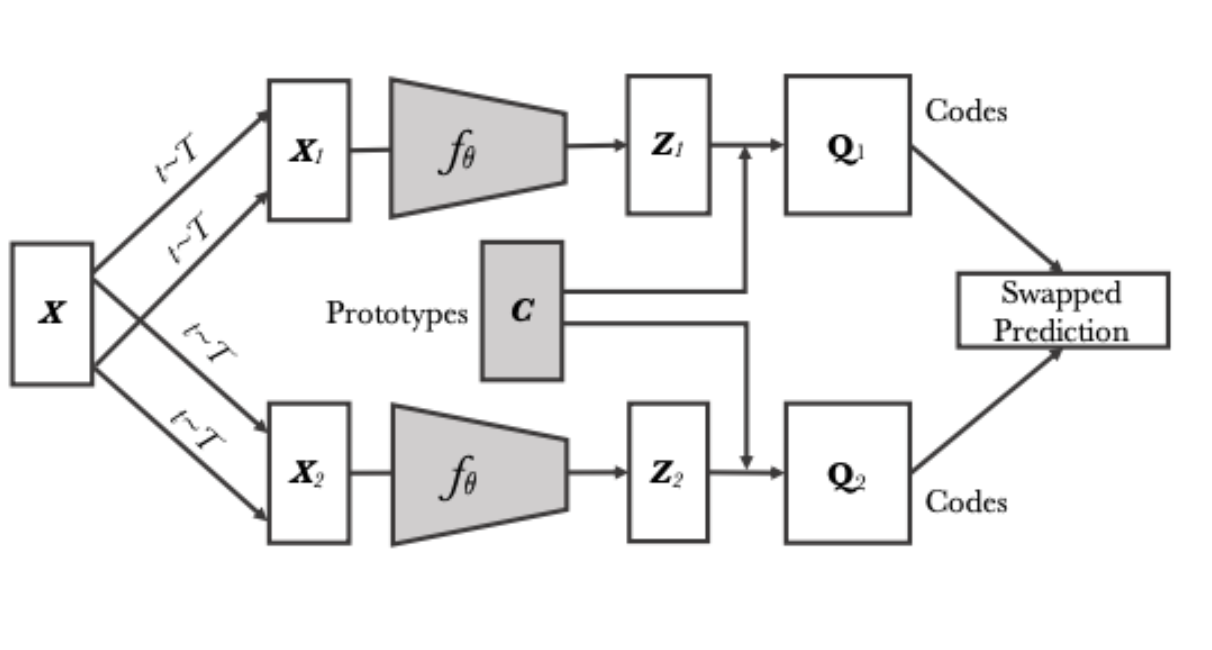
Creating Views:
- Take one image (x)
- Create two different augmented views: (v_1) and (v_2)
- Get their embeddings: (z_1 = f(v_1)) and (z_2 = f(v_2))
Clustering:
- Have a set of prototypes (C = {c_1, …, c_K})
- For each embedding, compute scores: (s = z^T C)
- Obtain soft assignments through the Sinkhorn-Knopp algorithm
Swapping Prediction:
- Predict assignments of the second view from the first and vice versa
- Loss function:
L = -\frac{1}{2}(Q_1 \log P_2 + Q_2 \log P_1)
where (Q) - target assignments, (P) - predicted assignments
Sinkhorn-Knopp Algorithm #
This algorithm ensures “uniform” clustering:
- Start with scores matrix (S)
- Iteratively normalize rows and columns:
Q = \text{diag}(u) \exp(S/\epsilon) \text{diag}(v) - Obtain balanced assignments
Counterfactual Explanations #
Counterfactual explanations answer the question “What needs to change to get a different result?”:
Optimization:
L_{cf} = -\log p(y_{target}|x_{cf}) + \lambda \|x_{cf} - x\|^2 + \lambda_{tv} TV(x_{cf})where:
- (x_{cf}) - counterfactual image
- (y_{target}) - target class
- (\lambda) - regularization coefficient
- (TV) - Total Variation regularization
Regularization:
- MSE loss maintains similarity with original
- Total Variation smooths changes
- L2 regularization prevents large changes
💻 Implementation #
Architecture #
SwAVModel
├── backbone: ResNet50
│   └── pretrained weights
├── projector: MLP
│   ├── Linear(2048 → 2048)
│   ├── BatchNorm + ReLU
│   ├── Linear(2048 → 2048)
│   ├── BatchNorm + ReLU
│   └── Linear(2048 → 512)
└── prototypes: Linear(512 → 50)
Dataset: Stanford Dogs #
We use the Stanford Dogs Dataset which consists of ~20K images across 120 breeds. This dataset is unlabeled in our pipeline, perfect for unsupervised learning.
The script automatically downloads and processes the dataset using torchvision’s ImageFolder:
from torchvision.datasets.utils import download_and_extract_archive

url = "http://vision.stanford.edu/aditya86/ImageNetDogs/images.tar"
download_and_extract_archive(url, download_root="./data")
Step 1: MultiCropTransform (Data Augmentation) #
Why? #
SwAV compares two views of the same image, so diverse augmentations are essential.
Use MultiCropTransform to generate two different views per image:
class MultiCropTransform:
    def __init__(self, base_transform):
        self.base_transform = base_transform

    def __call__(self, x):
        return [self.base_transform(x) for _ in range(2)]

transform = transforms.Compose([
    transforms.RandomResizedCrop(224),
    transforms.RandomHorizontalFlip(),
    transforms.ColorJitter(0.4, 0.4, 0.4, 0.1),
    transforms.ToTensor()
])
Step 2: Sinkhorn-Knopp Algorithm #
Why? #
To compute balanced cluster assignments from raw logits. It avoids degenerate solutions (e.g. all images in one cluster).
def sinkhorn(Q, n_iters=3, epsilon=0.05):
    Q = torch.exp(Q / epsilon).t()  # Transpose for row normalization
    Q /= Q.sum()

    K, B = Q.shape
    u = torch.zeros(K).to(Q.device)
    r = torch.ones(K).to(Q.device) / K
    c = torch.ones(B).to(Q.device) / B

    for _ in range(n_iters):
        u = Q.sum(dim=1)
        Q *= (r / u).unsqueeze(1)
        Q *= (c / Q.sum(dim=0)).unsqueeze(0)

    return (Q / Q.sum(dim=0, keepdim=True)).t()
Step 3: SwAV Model #
Components: #
- Backbone: ResNet50
- Projector: MLP for embedding projection
- Prototypes: Linear layer for cluster centers
class SwAVModel(nn.Module):
    def __init__(self, backbone, projection_dim, n_prototypes):
        super().__init__()
        self.backbone = backbone
        self.projector = nn.Sequential(
            nn.Linear(2048, 512),
            nn.ReLU(),
            nn.Linear(512, projection_dim)
        )
        self.prototypes = nn.Linear(projection_dim, n_prototypes, bias=False)

    def forward(self, x):
        feats = self.backbone(x)
        proj = self.projector(feats)
        proj = F.normalize(proj, dim=1)
        return self.prototypes(proj), proj
Step 4: Training Loop #
The loss combines prototype assignment similarity between two augmentations:
def train_swav(model, loader, optimizer):
    """
    One epoch of SwAV:
    - get two views: v1, v2
    - calculate embeddings and prototypes loggits
    - with sinkhorn get target assignments
    - minimize cross entropy
    """
    model.train()
    total_loss = 0.0

    # create progress bar
    pbar = tqdm(loader, desc='Training', leave=False)
    running_loss = 0.0

    for i, (images, _) in enumerate(pbar):
        images = [im.to(device) for im in images]

        z1, p1 = model(images[0])
        z2, p2 = model(images[1])
        with torch.no_grad():
            q1 = sinkhorn(p1)
            q2 = sinkhorn(p2)
        # SwAV loss: cross entropy
        loss = - (torch.sum(q2 * F.log_softmax(p1, dim=1), dim=1).mean()
                 + torch.sum(q1 * F.log_softmax(p2, dim=1), dim=1).mean()) * 0.5
        optimizer.zero_grad()
        loss.backward()
        optimizer.step()

        # update statistics
        total_loss += loss.item()
        running_loss = total_loss / (i + 1)

        # update bar
        pbar.set_postfix({'loss': f'{running_loss:.4f}'})

    return total_loss / len(loader)
SwAP training steps #
- Get Two Augmented Views:
The model processes two augmented views of the same image:
z1, p1 = model(images[0]): The first image generates embeddings (z1) and prototype logits (p1).
z2, p2 = model(images[1]): The second image generates embeddings (z2) and prototype logits (p2).
- Sinkhorn Normalization:
The Sinkhorn-Knopp algorithm is applied to the prototype logits to obtain target assignments:
q1 = sinkhorn(p1) for the first view.
q2 = sinkhorn(p2) for the second view.
- Loss Calculation (Cross-Entropy):
The SwAV loss is calculated using cross-entropy:
loss = - (torch.sum(q2 * F.log_softmax(p1, dim=1), dim=1).mean() + torch.sum(q1 * F.log_softmax(p2, dim=1), dim=1).mean()) * 0.5.
This loss function enforces the consistency of prototype assignments between the two augmented views.
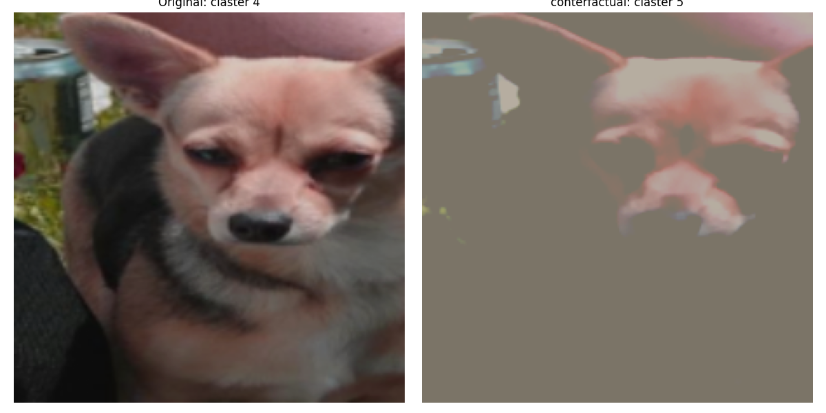
Step 5: Counterfactual Explanations #
Goal: #
“How should we change this image so that it belongs to another cluster?”
Algorithm by steps: #
Clone the image, make it ‘trainable’ (with requires_grad=True) - we will optimise it.
Run gradient descent to modify the image.
At each step:
We get p - probabilities of belonging to clusters.
We extract logit (confidence) on the target cluster target_proto.
We compute regularisations so as not to ‘break’ the image:
MSE: similarity to the original.
TV loss: smoothness of the image (no noise).
L2 norm: total deviation.
Calculating the total loss: the goal is to maximise the confidence of the model in the right cluster, while maintaining visual proximity.
We update the image via loss.backward() and optimiser.step().
We restrict the pixel values in the range [0, 1].
def generate_counterfactual(model, image, target_proto, lr=0.05, steps=300, lambda_reg=1.0, lambda_tv=0.1):
    """
    Generate counterfactual: change image so that it belongs to another cluster
    use gradient descent optimization with several regularization
    """
    model.eval()
    # clone image
    img_cf = image.clone().detach().to(device).requires_grad_(True)
    optimizer = optim.Adam([img_cf], lr=lr)

    # calculate Total Variation loss
    def tv_loss(img):
        diff_h = torch.abs(img[:, :, 1:, :] - img[:, :, :-1, :]).sum()
        diff_w = torch.abs(img[:, :, :, 1:] - img[:, :, :, :-1]).sum()
        return (diff_h + diff_w) / (img.shape[2] * img.shape[3])

    for i in range(steps):
        _, p = model(img_cf)
        # loggit of prototype
        proto_logit = p[:, target_proto].mean()

        # regularization
        reg_loss = F.mse_loss(img_cf, image.to(device))

        tv_reg = tv_loss(img_cf)

        # L2 regularization
        l2_reg = torch.norm(img_cf - image.to(device))

        # maximize proto_logit
        loss = -proto_logit + lambda_reg * reg_loss + lambda_tv * tv_reg + 0.01 * l2_reg

        optimizer.zero_grad()
        loss.backward()
        optimizer.step()

        # constraints pizels values
        img_cf.data.clamp_(0, 1)

        # print progress
        if (i+1) % 50 == 0:
            print(f"Step {i+1}/{steps}, Loss: {loss.item():.4f}, Proto logit: {proto_logit.item():.4f}")

    return img_cf.detach()
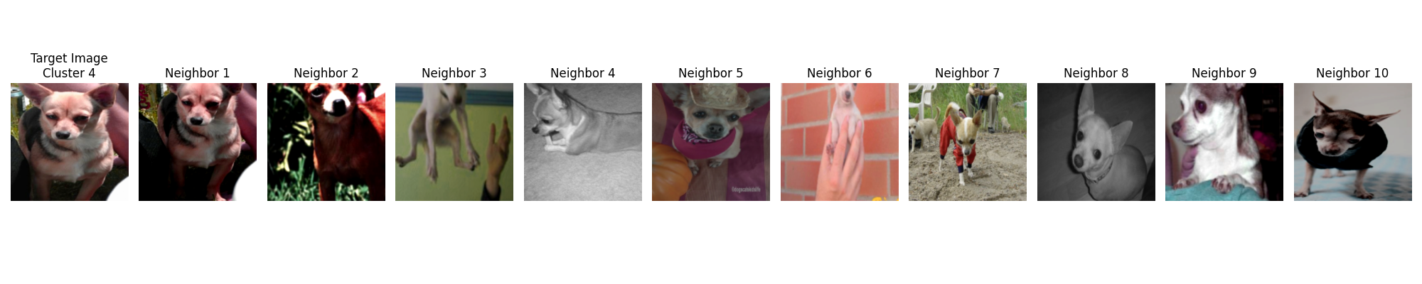
Step 6: Visualizing Clusters #
def visualize_cluster_members(embeddings, cluster_labels, query_idx, k=5):
    from sklearn.metrics.pairwise import cosine_similarity

    query = embeddings[query_idx].reshape(1, -1)
    sims = cosine_similarity(query, embeddings)[0]
    topk = sims.argsort()[-k:][::-1]

    fig, axes = plt.subplots(1, k, figsize=(15, 4))
    for i, idx in enumerate(topk):
        axes[i].imshow(load_image_by_index(idx))
        axes[i].axis('off')
    plt.show()
Results #
Clasters example
Conterfactual example
 #
#
Future Tips #
- Try different number of prototypes (clusters)
- Extend to StyleGAN2-generated counterfactuals
Install Dependencies: #
pip install torch torchvision tqdm matplotlib numpy Pillow requests
Why XAI Matters #
Explainability bridges the gap between black-box deep learning and trustworthy AI. With counterfactuals, we can:
- Understand what makes an image belong to a cluster
- Explore decision boundaries
- Generate interpretable visual feedback